MultiLayer Awesome Oscillator Saucer Strategy [Skyrexio]Overview
MultiLayer Awesome Oscillator Saucer Strategy leverages the combination of Awesome Oscillator (AO), Williams Alligator, Williams Fractals and Exponential Moving Average (EMA) to obtain the high probability long setups. Moreover, strategy uses multi trades system, adding funds to long position if it considered that current trend has likely became stronger. Awesome Oscillator is used for creating signals, while Alligator and Fractal are used in conjunction as an approximation of short-term trend to filter them. At the same time EMA (default EMA's period = 100) is used as high probability long-term trend filter to open long trades only if it considers current price action as an uptrend. More information in "Methodology" and "Justification of Methodology" paragraphs. The strategy opens only long trades.
Unique Features
No fixed stop-loss and take profit: Instead of fixed stop-loss level strategy utilizes technical condition obtained by Fractals and Alligator to identify when current uptrend is likely to be over (more information in "Methodology" and "Justification of Methodology" paragraphs)
Configurable Trading Periods: Users can tailor the strategy to specific market windows, adapting to different market conditions.
Multilayer trades opening system: strategy uses only 10% of capital in every trade and open up to 5 trades at the same time if script consider current trend as strong one.
Short and long term trend trade filters: strategy uses EMA as high probability long-term trend filter and Alligator and Fractal combination as a short-term one.
Methodology
The strategy opens long trade when the following price met the conditions:
1. Price closed above EMA (by default, period = 100). Crossover is not obligatory.
2. Combination of Alligator and Williams Fractals shall consider current trend as an upward (all details in "Justification of Methodology" paragraph)
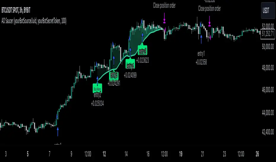
3. Awesome Oscillator shall create the "Saucer" long signal (all details in "Justification of Methodology" paragraph). Buy stop order is placed one tick above the candle's high of last created "Saucer signal".
4. If price reaches the order price, long position is opened with 10% of capital.
5. If currently we have opened position and price creates and hit the order price of another one "Saucer" signal another one long position will be added to the previous with another one 10% of capital. Strategy allows to open up to 5 long trades simultaneously.
6. If combination of Alligator and Williams Fractals shall consider current trend has been changed from up to downtrend, all long trades will be closed, no matter how many trades has been opened.
Script also has additional visuals. If second long trade has been opened simultaneously the Alligator's teeth line is plotted with the green color. Also for every trade in a row from 2 to 5 the label "Buy More" is also plotted just below the teeth line. With every next simultaneously opened trade the green color of the space between teeth and price became less transparent.
Strategy settings
In the inputs window user can setup strategy setting: EMA Length (by default = 100, period of EMA, used for long-term trend filtering EMA calculation). User can choose the optimal parameters during backtesting on certain price chart.
Justification of Methodology
Let's go through all concepts used in this strategy to understand how they works together. Let's start from the easies one, the EMA. Let's briefly explain what is EMA. The Exponential Moving Average (EMA) is a type of moving average that gives more weight to recent prices, making it more responsive to current price changes compared to the Simple Moving Average (SMA). It is commonly used in technical analysis to identify trends and generate buy or sell signals. It can be calculated with the following steps:
1.Calculate the Smoothing Multiplier:
Multiplier = 2 / (n + 1), Where n is the number of periods.
2. EMA Calculation
EMA = (Current Price) × Multiplier + (Previous EMA) × (1 − Multiplier)
In this strategy uses EMA an initial long term trend filter. It allows to open long trades only if price close above EMA (by default 50 period). It increases the probability of taking long trades only in the direction of the trend.
Let's go to the next, short-term trend filter which consists of Alligator and Fractals. Let's briefly explain what do these indicators means. The Williams Alligator, developed by Bill Williams, is a technical indicator designed to spot trends and potential market reversals. It uses three smoothed moving averages, referred to as the jaw, teeth, and lips:
Jaw (Blue Line): The slowest of the three, based on a 13-period smoothed moving average shifted 8 bars ahead.
Teeth (Red Line): The medium-speed line, derived from an 8-period smoothed moving average shifted 5 bars forward.
Lips (Green Line): The fastest line, calculated using a 5-period smoothed moving average shifted 3 bars forward.
When these lines diverge and are properly aligned, the "alligator" is considered "awake," signaling a strong trend. Conversely, when the lines overlap or intertwine, the "alligator" is "asleep," indicating a range-bound or sideways market. This indicator assists traders in identifying when to act on or avoid trades.
The Williams Fractals, another tool introduced by Bill Williams, are used to pinpoint potential reversal points on a price chart. A fractal forms when there are at least five consecutive bars, with the middle bar displaying the highest high (for an up fractal) or the lowest low (for a down fractal), relative to the two bars on either side.
Key Points:
Up Fractal: Occurs when the middle bar has a higher high than the two preceding and two following bars, suggesting a potential downward reversal.
Down Fractal: Happens when the middle bar shows a lower low than the surrounding two bars, hinting at a possible upward reversal.
Traders often combine fractals with other indicators to confirm trends or reversals, improving the accuracy of trading decisions.
How we use their combination in this strategy? Let’s consider an uptrend example. A breakout above an up fractal can be interpreted as a bullish signal, indicating a high likelihood that an uptrend is beginning. Here's the reasoning: an up fractal represents a potential shift in market behavior. When the fractal forms, it reflects a pullback caused by traders selling, creating a temporary high. However, if the price manages to return to that fractal’s high and break through it, it suggests the market has "changed its mind" and a bullish trend is likely emerging.
The moment of the breakout marks the potential transition to an uptrend. It’s crucial to note that this breakout must occur above the Alligator's teeth line. If it happens below, the breakout isn’t valid, and the downtrend may still persist. The same logic applies inversely for down fractals in a downtrend scenario.
So, if last up fractal breakout was higher, than Alligator's teeth and it happened after last down fractal breakdown below teeth, algorithm considered current trend as an uptrend. During this uptrend long trades can be opened if signal was flashed. If during the uptrend price breaks down the down fractal below teeth line, strategy considered that uptrend is finished with the high probability and strategy closes all current long trades. This combination is used as a short term trend filter increasing the probability of opening profitable long trades in addition to EMA filter, described above.
Now let's talk about Awesome Oscillator's "Sauser" signals. Briefly explain what is the Awesome Oscillator. The Awesome Oscillator (AO), created by Bill Williams, is a momentum-based indicator that evaluates market momentum by comparing recent price activity to a broader historical context. It assists traders in identifying potential trend reversals and gauging trend strength.
AO = SMA5(Median Price) − SMA34(Median Price)
where:
Median Price = (High + Low) / 2
SMA5 = 5-period Simple Moving Average of the Median Price
SMA 34 = 34-period Simple Moving Average of the Median Price
Now we know what is AO, but what is the "Saucer" signal? This concept was introduced by Bill Williams, let's briefly explain it and how it's used by this strategy. Initially, this type of signal is a combination of the following AO bars: we need 3 bars in a row, the first one shall be higher than the second, the third bar also shall be higher, than second. All three bars shall be above the zero line of AO. The price bar, which corresponds to third "saucer's" bar is our signal bar. Strategy places buy stop order one tick above the price bar which corresponds to signal bar.
After that we can have the following scenarios.
Price hit the order on the next candle in this case strategy opened long with this price.
Price doesn't hit the order price, the next candle set lower low. If current AO bar is increasing buy stop order changes by the script to the high of this new bar plus one tick. This procedure repeats until price finally hit buy order or current AO bar become decreasing. In the second case buy order cancelled and strategy wait for the next "Saucer" signal.
If long trades has been opened strategy use all the next signals until number of trades doesn't exceed 5. All trades are closed when the trend changes to downtrend according to combination of Alligator and Fractals described above.
Why we use "Saucer" signals? If AO above the zero line there is a high probability that price now is in uptrend if we take into account our two trend filters. When we see the decreasing bars on AO and it's above zero it's likely can be considered as a pullback on the uptrend. When we see the stop of AO decreasing and the first increasing bar has been printed there is a high probability that this local pull back is finished and strategy open long trade in the likely direction of a main trend.
Why strategy use only 10% per signal? Sometimes we can see the false signals which appears on sideways. Not risking that much script use only 10% per signal. If the first long trade has been open and price continue going up and our trend approximation by Alligator and Fractals is uptrend, strategy add another one 10% of capital to every next saucer signal while number of active trades no more than 5. This capital allocation allows to take part in long trades when current uptrend is likely to be strong and use only 10% of capital when there is a high probability of sideways.
Backtest Results
Operating window: Date range of backtests is 2023.01.01 - 2024.11.25. It is chosen to let the strategy to close all opened positions.
Commission and Slippage: Includes a standard Binance commission of 0.1% and accounts for possible slippage over 5 ticks.
Initial capital: 10000 USDT
Percent of capital used in every trade: 10%
Maximum Single Position Loss: -5.10%
Maximum Single Profit: +22.80%
Net Profit: +2838.58 USDT (+28.39%)
Total Trades: 107 (42.99% win rate)
Profit Factor: 3.364
Maximum Accumulated Loss: 373.43 USDT (-2.98%)
Average Profit per Trade: 26.53 USDT (+2.40%)
Average Trade Duration: 78 hours
These results are obtained with realistic parameters representing trading conditions observed at major exchanges such as Binance and with realistic trading portfolio usage parameters.
How to Use
Add the script to favorites for easy access.
Apply to the desired timeframe and chart (optimal performance observed on 3h BTC/USDT).
Configure settings using the dropdown choice list in the built-in menu.
Set up alerts to automate strategy positions through web hook with the text: {{strategy.order.alert_message}}
Disclaimer:
Educational and informational tool reflecting Skyrex commitment to informed trading. Past performance does not guarantee future results. Test strategies in a simulated environment before live implementation
Cari dalam skrip untuk "the strat"
Fractional Accumulation Distribution Strategy🔹 INTRODUCTION:
As traders and investors, we often find ourselves searching for ways to maximize our market positioning—trying to capture the best price, manage risk, and adapt to ever-changing volatility. Through years of working with a variety of traders and investors, a common theme emerged: the most successful market participants were those who accumulated positions strategically over time, rather than relying on one-off, rigid entry points. However, even the best of them struggled to consistently time their entries and exits for optimal results.
That's why I created the Fractional Accumulation/Distribution Strategy (FADS)—an adaptable solution designed to dynamically adjust position sizing and entry points based on changing market conditions, enabling both passive and active market participants to optimize their approach.
The FADS trading strategy combines volatility-based trend detection and adaptive position scaling to maximize profitability across varied market conditions. By using the price ranges from higher timeframes, FADS pinpoints extreme demand and supply zones with a high statistical probability of reversal, making it effective in both high and low volatility environments. By applying adjustable threshold settings, users can focus on meaningful price movements to reduce unnecessary trades. Adaptive position scaling further enhances this approach by adjusting position sizes based on entry level distances, allowing for strategic position building that balances risk and reward in uncertain markets. This systematic scaling begins with smaller positions, expanding as the trend solidifies, creating a refined, robust trading experience.
🔹 FEATURES:
Multi-Timeframe Volatility-Based Trend Detection
Accumulation/Distribution Level Filter
Customizable Period for Highest/Lowest Prices Capture
Adjustable Sensitivity & Frequency in Positioning
Broad control settings of Strategy
Adaptive Position Scaling
🔹 SETTINGS:
Volatility : Determines trading range based on market volatility . Highest range value number of periods.
Factor : Adjusts the width of the Accumulation & Distribution bands separately. The Level Filter feature offers customizable triggering bands, allowing users to fine-tune the initiation point for the Accumulation/Distribution sequence. This flexibility enables traders to align entries more precisely with market conditions, setting optimal thresholds for initiating trade chains, whether in accumulating positions during uptrends or distributing in downtrends.
Lowest : Choose the price source (e.g., Close, Low). Number of bars considered when determining the lowest price level. Selecting the checkbox generate a signal when the price crosses below the previous lowest value for calculating the lowest value used for trade signals.
Highest : Choose the price source (e.g., Close, High). Number of bars considered when determining the highest price levels. Selecting the checkbox generate a signal when the price crosses above the previous highest value for calculating the highest value used for trade signals.
Accumulation Spread : Adjusts the buying frequency sensitivity by setting the distance between entries based on personal risk tolerance. Larger values for less frequent buys; smaller values for more frequent buys.
Distribution Spread : Adjusts the selling frequency sensitivity by setting the distance between exits based on reward preference. Larger values for less frequent sells; smaller values for more frequent sells.
Percentage of Capital Allocation : Sets the portion of total capital used for the initial trade in a strategy. It sets the scale for subsequent trades during accumulation phase.
🔹 APPLICATIONS:
❖ Accumulation and Distribution Phases
Early entries are avoided by initiating accumulation only after a trend reversal is confirmed and price breaks below long-term range.
Position sizes are determined by the distance between consecutive trades, smaller distance results in smaller position sizes and vice versa.
Average position cost is reduced by accumulating larger positions at the lower prices, potentially resulting in improved profitability.
Early exits are avoided by initiating distribution only after trend reversal is confirmed and price breaks above long-term range.
The pace of distribution can be tracked by the violet line that represents average positions during distribution phase
❖ Use Cases (Different than default setting input is used for illustration purposes)
If the starting point of accumulation starts too high for the risk preference, Accumulation Level Filter can be lowered by increasing the 🟢 threshold Factor.
If the starting point of distribution is too low for the reward preference, the Distribution Level Filter can be raised by increasing the 🔴 threshold Factor.
In lower timeframes, positions during the accumulation phase could be purchased at higher levels relative to prior entry positions. To optimize for this, consider extending the period used to capture the lowest prices. Similarly, during the distribution phase, increasing the period for identifying higher prices can improve accuracy.
🔹 Strategy Properties:
Adjusting properties within the script settings is recommended to align with specific accounts and trading platforms, ensuring realistic strategy results.
Balance (default): $100,000
Initial Order Size: 1% of the default balance
Commission: 0.1%
Slippage: 5 Ticks
Backtesting: Backtested using TradingView’s built-in strategy testing tool with default commission rates of 0.1% and slippage of 5 ticks. It reflects average market conditions for Apple Inc. (APPL) on 1-hour timeframe
Disclaimers: Commission and slippage varies with market conditions and brokerage policies. The assumed value may not represent all trading environments.
PAST PERFORMANCE DOESN’T GUARANTEE FUTURE RESULTS!
Disclaimer: Please remember that past performance may not be indicative of future results. Due to various factors, including changing market conditions, the strategy may no longer perform as well as in historical backtesting. This post and the script don’t provide any financial advice.
This invite-only script is being published as part of my commitment to developing tools that align with TradingView’s community standards. Access requests will be reviewed carefully after the script passes TradingView's moderation process.

SuperATR 7-Step Profit - Strategy [presentTrading] Long time no see!
█ Introduction and How It Is Different
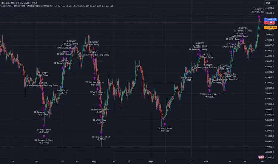
The SuperATR 7-Step Profit Strategy is a multi-layered trading approach that integrates adaptive Average True Range (ATR) calculations with momentum-based trend detection. What sets this strategy apart is its sophisticated 7-step take-profit mechanism, which combines four ATR-based exit levels and three fixed percentage levels. This hybrid approach allows traders to dynamically adjust to market volatility while systematically capturing profits in both long and short market positions.
Traditional trading strategies often rely on static indicators or single-layered exit strategies, which may not adapt well to changing market conditions. The SuperATR 7-Step Profit Strategy addresses this limitation by:
- Using Adaptive ATR: Enhances the standard ATR by making it responsive to current market momentum.
- Incorporating Momentum-Based Trend Detection: Identifies stronger trends with higher probability of continuation.
- Employing a Multi-Step Take-Profit System: Allows for gradual profit-taking at predetermined levels, optimizing returns while minimizing risk.
BTCUSD 6hr Performance
█ Strategy, How It Works: Detailed Explanation
The strategy revolves around detecting strong market trends and capitalizing on them using an adaptive ATR and momentum indicators. Below is a detailed breakdown of each component of the strategy.
🔶 1. True Range Calculation with Enhanced Volatility Detection
The True Range (TR) measures market volatility by considering the most significant price movements. The enhanced TR is calculated as:
TR = Max
Where:
High and Low are the current bar's high and low prices.
Previous Close is the closing price of the previous bar.
Abs denotes the absolute value.
Max selects the maximum value among the three calculations.
🔶 2. Momentum Factor Calculation
To make the ATR adaptive, the strategy incorporates a Momentum Factor (MF), which adjusts the ATR based on recent price movements.
Momentum = Close - Close
Stdev_Close = Standard Deviation of Close over n periods
Normalized_Momentum = Momentum / Stdev_Close (if Stdev_Close ≠ 0)
Momentum_Factor = Abs(Normalized_Momentum)
Where:
Close is the current closing price.
n is the momentum_period, a user-defined input (default is 7).
Standard Deviation measures the dispersion of closing prices over n periods.
Abs ensures the momentum factor is always positive.
🔶 3. Adaptive ATR Calculation
The Adaptive ATR (AATR) adjusts the traditional ATR based on the Momentum Factor, making it more responsive during volatile periods and smoother during consolidation.
Short_ATR = SMA(True Range, short_period)
Long_ATR = SMA(True Range, long_period)
Adaptive_ATR = /
Where:
SMA is the Simple Moving Average.
short_period and long_period are user-defined inputs (defaults are 3 and 7, respectively).
🔶 4. Trend Strength Calculation
The strategy quantifies the strength of the trend to filter out weak signals.
Price_Change = Close - Close
ATR_Multiple = Price_Change / Adaptive_ATR (if Adaptive_ATR ≠ 0)
Trend_Strength = SMA(ATR_Multiple, n)
🔶 5. Trend Signal Determination
If (Short_MA > Long_MA) AND (Trend_Strength > Trend_Strength_Threshold):
Trend_Signal = 1 (Strong Uptrend)
Elif (Short_MA < Long_MA) AND (Trend_Strength < -Trend_Strength_Threshold):
Trend_Signal = -1 (Strong Downtrend)
Else:
Trend_Signal = 0 (No Clear Trend)
🔶 6. Trend Confirmation with Price Action
Adaptive_ATR_SMA = SMA(Adaptive_ATR, atr_sma_period)
If (Trend_Signal == 1) AND (Close > Short_MA) AND (Adaptive_ATR > Adaptive_ATR_SMA):
Trend_Confirmed = True
Elif (Trend_Signal == -1) AND (Close < Short_MA) AND (Adaptive_ATR > Adaptive_ATR_SMA):
Trend_Confirmed = True
Else:
Trend_Confirmed = False
Local Performance
🔶 7. Multi-Step Take-Profit Mechanism
The strategy employs a 7-step take-profit system
█ Trade Direction
The SuperATR 7-Step Profit Strategy is designed to work in both long and short market conditions. By identifying strong uptrends and downtrends, it allows traders to capitalize on price movements in either direction.
Long Trades: Initiated when the market shows strong upward momentum and the trend is confirmed.
Short Trades: Initiated when the market exhibits strong downward momentum and the trend is confirmed.
█ Usage
To implement the SuperATR 7-Step Profit Strategy:
1. Configure the Strategy Parameters:
- Adjust the short_period, long_period, and momentum_period to match the desired sensitivity.
- Set the trend_strength_threshold to control how strong a trend must be before acting.
2. Set Up the Multi-Step Take-Profit Levels:
- Define ATR multipliers and fixed percentage levels according to risk tolerance and profit goals.
- Specify the percentage of the position to close at each level.
3. Apply the Strategy to a Chart:
- Use the strategy on instruments and timeframes where it has been tested and optimized.
- Monitor the positions and adjust parameters as needed based on performance.
4. Backtest and Optimize:
- Utilize TradingView's backtesting features to evaluate historical performance.
- Adjust the default settings to optimize for different market conditions.
█ Default Settings
Understanding default settings is crucial for optimal performance.
Short Period (3): Affects the responsiveness of the short-term MA.
Effect: Lower values increase sensitivity but may produce more false signals.
Long Period (7): Determines the trend baseline.
Effect: Higher values reduce noise but may delay signals.
Momentum Period (7): Influences adaptive ATR and trend strength.
Effect: Shorter periods react quicker to price changes.
Trend Strength Threshold (0.5): Filters out weaker trends.
Effect: Higher thresholds yield fewer but stronger signals.
ATR Multipliers: Set distances for ATR-based exits.
Effect: Larger multipliers aim for bigger moves but may reduce hit rate.
Fixed TP Levels (%): Control profit-taking on smaller moves.
Effect: Adjusting these levels affects how quickly profits are realized.
Exit Percentages: Determine how much of the position is closed at each TP level.
Effect: Higher percentages reduce exposure faster, affecting risk and reward.
Adjusting these variables allows you to tailor the strategy to different market conditions and personal risk preferences.
By integrating adaptive indicators and a multi-tiered exit strategy, the SuperATR 7-Step Profit Strategy offers a versatile tool for traders seeking to navigate varying market conditions effectively. Understanding and adjusting the key parameters enables traders to harness the full potential of this strategy.
Keltner Channel Strategy by Kevin DaveyKeltner Channel Strategy Description
The Keltner Channel Strategy is a volatility-based trading approach that uses the Keltner Channel, a technical indicator derived from the Exponential Moving Average (EMA) and Average True Range (ATR). The strategy helps identify potential breakout or mean-reversion opportunities in the market by plotting upper and lower bands around a central EMA, with the channel width determined by a multiplier of the ATR.
Components:
1. Exponential Moving Average (EMA):
The EMA smooths price data by placing greater weight on recent prices, allowing traders to track the market’s underlying trend more effectively than a simple moving average (SMA). In this strategy, a 20-period EMA is used as the midline of the Keltner Channel.
2. Average True Range (ATR):
The ATR measures market volatility over a 14-period lookback. By calculating the average of the true ranges (the greatest of the current high minus the current low, the absolute value of the current high minus the previous close, or the absolute value of the current low minus the previous close), the ATR captures how much an asset typically moves over a given period.
3. Keltner Channel:
The upper and lower boundaries are set by adding or subtracting 1.5 times the ATR from the EMA. These boundaries create a dynamic range that adjusts with market volatility.
Trading Logic:
• Long Entry Condition: The strategy enters a long position when the closing price falls below the lower Keltner Channel, indicating a potential buying opportunity at a support level.
• Short Entry Condition: The strategy enters a short position when the closing price exceeds the upper Keltner Channel, signaling a potential selling opportunity at a resistance level.
The strategy plots the upper and lower Keltner Channels and the EMA on the chart, providing a visual representation of support and resistance levels based on market volatility.
Scientific Support for Volatility-Based Strategies:
The use of volatility-based indicators like the Keltner Channel is supported by numerous studies on price momentum and volatility trading. Research has shown that breakout strategies, particularly those leveraging volatility bands such as the Keltner Channel or Bollinger Bands, can be effective in capturing trends and reversals in both trending and mean-reverting markets  .
Who is Kevin Davey?
Kevin Davey is a highly respected algorithmic trader, author, and educator, known for his systematic approach to building and optimizing trading strategies. With over 25 years of experience in the markets, Davey has earned a reputation as an expert in quantitative and rule-based trading. He is particularly well-known for winning several World Cup Trading Championships, where he consistently demonstrated high returns with low risk.

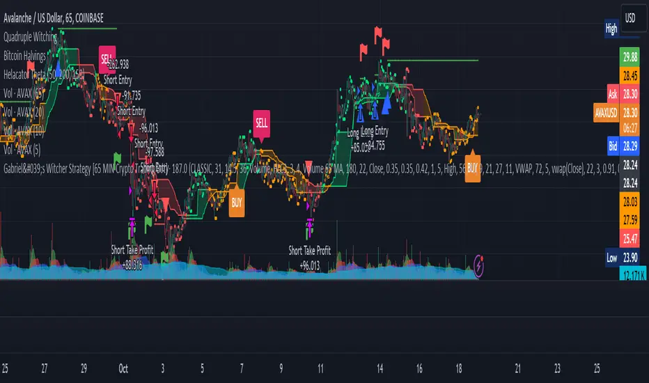
Gabriel's Witcher Strategy [65 Minute Trading Bot]Strategy Description: Gabriel's Witcher Strategy
Author: Gabriel
Platform: TradingView Pine Script (Version 5)
Backtested Asset: Avalanche (Coinbase Brokage for Volume adjustment)
Timeframe: 65 Minutes
Strategy Type: Comprehensive Trend-Following and Momentum Strategy with Scalping and Risk Management Features
Overview
Gabriel's Witcher Strategy is an advanced trading bot designed for the Avalanche pair on a 65-minute timeframe. This strategy integrates a multitude of technical indicators to identify and execute high-probability trading opportunities. By combining trend-following, momentum, volume analysis, and range filtering, the strategy aims to capitalize on both long and short market movements. Additionally, it incorporates scalping mechanisms and robust risk management features, including take-profit (TP) levels and commission considerations, to optimize trade performance and profitability.
====Key Components====
Source Selection:
Custom Source Flexibility: Allows traders to select from a wide range of price and volume sources (e.g., Close, Open, High, Low, HL2, HLC3, OHLC4, VWAP, On-Balance Volume, etc.) for indicator calculations, enhancing adaptability to various trading styles.
Various curves of Volume Analysis are employed:
Tick Volume Calculation: Utilizes tick volume as a fallback when actual volume data is unavailable, ensuring consistency across different data feeds.
Volume Indicators: Incorporates multiple volume-based indicators such as On-Balance Volume (OBV), Accumulation/Distribution (AccDist), Negative Volume Index (NVI), Positive Volume Index (PVI), and Price Volume Trend (PVT) for comprehensive market analysis.
Trend Indicators:
ADX (Average Directional Index): Measures trend strength using either the Classic or Masanakamura method, with customizable length and threshold settings. It's used to open positions when the mesured trend is strong, or exit when its weak.
Jurik Moving Average (JMA): A smooth moving average that reduces lag, configurable with various parameters including source, resolution, and repainting options.
Parabolic SAR: Identifies potential reversals in market trends with adjustable start, increment, and maximum settings.
Custom Trend Indicator: Utilizes highest and lowest price points over a specified timeframe to determine current and previous trend bases, visually represented with color-filled areas.
Momentum Indicators:
Relative Strength Index (RSI): Evaluates the speed and change of price movements, smoothed with a custom length and source. It's used to not enter the market for shorts in oversold or longs for overbought conditions, and to enter for long in oversold or shorts for overboughts.
Momentum-Based Calculations: Employs both Double Exponential Moving Averages (DEMA) on a MACD-based RSI to enhance momentum signal accuracy which is then further accelerated by a Hull MA. This is the technical analysis tool that determines bearish or bullish momentum.
OBV-Based Momentum Conditions: Uses two exponential moving averages of OBV to determine bullish or bearish momentum shifts, anomalities, breakouts where banks flow their funds in or Smart Money Concepts trade.
Moving Averages (MA):
Multiple MA Types: Includes Simple Moving Average (SMA), Exponential Moving Average (EMA), Weighted Moving Average (WMA), Hull Moving Average (HMA), and Volume-Weighted Moving Average (VWMA), selectable via input parameters.
MA Speed Calculation: Measures the percentage change in MA values to determine the direction and speed of the trend.
Range Filtering:
Variance-Based Filter: Utilizes variance and moving averages to filter out trades during low-volatility periods, enhancing trade quality.
Color-Coded Range Indicators: Visualizes range filtering with color changes on the chart for quick assessment.
Scalping Mechanism:
Heikin-Ashi Candles: Optionally uses Heikin-Ashi candles for smoother price action analysis.
EMA-Based Trend Detection: Employs fast, medium, and slow EMAs to determine trend direction and potential entry points.
Fractal-Based Filtering: Detects regular or BW (Black & White) fractals to confirm trade signals.
Take Profit (TP) Management:
Dynamic TP Levels: Calculates TP levels based on the number of consecutive long or short entries, adjusting targets to maximize profits.
TP Signals and Re-Entry: Plots TP signals on the chart and allows for automatic re-entry upon TP hit, maintaining continuous trade flow.
Risk Management:
Commission Integration: Accounts for trading commissions to ensure net profitability.
Position Sizing: Configured to use a percentage of equity for each trade, adjustable via input parameters.
Pyramiding: Allows up to one additional position per direction to enhance gains during strong trends.
Alerts and Visual Indicators:
Buy/Sell Signals: Plots visual indicators (triangles and flags) on the chart to signify entry and TP points.
Bar Coloring: Changes bar colors based on ADX and trend conditions for immediate visual cues.
Price Levels: Marks significant price levels related to TP and position entries with cross styles.
Input Parameters
Source Settings:
Custom Sources (srcinput): Choose from various price and volume sources to tailor indicator calculations.
ADX Settings:
ADX Type (ADX_options): Select between 'CLASSIC' and 'MASANAKAMURA' methods.
ADX Length (ADX_len): Defines the period for ADX calculation.
ADX Threshold (th): Sets the minimum ADX value to consider a strong trend.
RSI Settings:
RSI Length (len_3): Period for RSI calculation.
RSI Source (src_3): Source data for RSI.
Trend Strength Settings:
Channel Length (n1): Period for trend channel calculation.
Average Length (n2): Period for smoothing trend strength.
Jurik Moving Average (JMA) Settings:
JMA Source (inp): Source data for JMA.
JMA Resolution (reso): Timeframe for JMA calculation.
JMA Repainting (rep): Option to allow JMA to repaint.
JMA Length (lengths): Period for JMA.
Parabolic SAR Settings:
SAR Start (start): Initial acceleration factor.
SAR Increment (increment): Acceleration factor increment.
SAR Maximum (maximum): Maximum acceleration factor.
SAR Point Width (width): Visual width of SAR points.
Trend Indicator Settings:
Trend Timeframe (timeframe): Period for trend indicator calculations.
Momentum Settings:
Source Type (srcType): Select between 'Price' and 'VWAP'.
Momentum Source (srcPrice): Source data for momentum calculations.
RSI Length (rsiLen): Period for momentum RSI.
Smooth Length (sLen): Smoothing period for momentum RSI.
OBV Settings:
OBV Line 1 (e1): EMA period for OBV line 1.
OBV Line 2 (e2): EMA period for OBV line 2.
Moving Average (MA) Settings:
MA Length (length): Period for MA calculations.
MA Type (matype): Select MA type (1: SMA, 2: EMA, 3: HMA, 4: WMA, 5: VWMA).
Range Filter Settings:
Range Filter Length (length0): Period for range filtering.
Range Filter Multiplier (mult): Multiplier for range variance.
Take Profit (TP) Settings:
TP Long (tp_long0): Percentage for long TP.
TP Short (tp_short0): Percentage for short TP.
Scalping Settings:
Scalping Activation (ACT_SCLP): Enable or disable scalping.
Scalping Length (HiLoLen): Period for scalping indicators.
Fast EMA Length (fastEMAlength): Period for fast EMA in scalping.
Medium EMA Length (mediumEMAlength): Period for medium EMA in scalping.
Slow EMA Length (slowEMAlength): Period for slow EMA in scalping.
Filter (filterBW): Enable or disable additional fractal filtering.
Pullback Lookback (Lookback): Number of bars for pullback consideration.
Use Heikin-Ashi Candles (UseHAcandles): Option to use Heikin-Ashi candles for smoother trend analysis.
Strategy Logic
Indicator Calculations:
Volume and Source Selection: Determines the primary data source based on user input, ensuring flexibility and adaptability.
ADX Calculation: Computes ADX using either the Classic or Masanakamura method to assess trend strength.
RSI Calculation: Evaluates market momentum using RSI, further smoothed with custom periods.
Trend Strength Assessment: Utilizes trend channel and average lengths to gauge the robustness of current trends.
Jurik Moving Average (JMA): Smooths price data to reduce lag and enhance trend detection.
Parabolic SAR: Identifies potential trend reversals with adjustable parameters for sensitivity.
Momentum Analysis: Combines RSI with DEMA and OBV-based conditions to confirm bullish or bearish momentum.
Moving Averages: Employs multiple MA types to determine trend direction and speed.
Range Filtering: Filters out low-volatility periods to focus on high-probability trades.
Trade Conditions:
Long Entry Conditions:
ADX Confirmation: ADX must be above the threshold, indicating a strong uptrend.
RSI and Momentum: RSI below 70 and positive momentum signals.
JMA and SAR: JMA indicates an uptrend, and Parabolic SAR is below the price.
Trend Indicator: Confirms the current trend direction.
Range Filter: Ensures market is in an upward range.
Scalping Option: If enabled, additional scalping conditions must be met.
Short Entry Conditions:
ADX Confirmation: ADX must be above the threshold, indicating a strong downtrend.
RSI and Momentum: RSI above 30 and negative momentum signals.
JMA and SAR: JMA indicates a downtrend, and Parabolic SAR is above the price.
Trend Indicator: Confirms the current trend direction.
Range Filter: Ensures market is in a downward range.
Scalping Option: If enabled, additional scalping conditions must be met.
Position Management:
Entry Execution: Places long or short orders based on the identified conditions and user-selected position types (Longs, Shorts, or Both).
Take Profit (TP): Automatically sets TP levels based on predefined percentages, adjusting dynamically with consecutive trades.
Re-Entry Mechanism: Allows for automatic re-entry upon TP hit, maintaining active trading positions.
Exit Conditions: Closes positions when TP levels are reached or when opposing trend signals are detected.
Visual Indicators:
Bar Coloring: Highlights bars in green for bullish conditions, red for bearish, and orange for neutral.
Plotting Price Levels: Marks significant price levels related to TP and trade entries with cross symbols.
Signal Shapes: Displays triangle and flag shapes on the chart to indicate trade entries and TP hits.
Alerts:
Custom Alerts: Configured to notify traders of long entries, short entries, and TP hits, enabling timely trade management and execution.
Usage Instructions
Setup:
Apply the Strategy: Add the script to your TradingView chart set to BTCUSDT with a 65-minute timeframe.
Configure Inputs: Adjust the input parameters under their respective groups (e.g., Source Settings, ADX, RSI, Trend Strength, etc.) to match your trading preferences and risk tolerance.
Position Selection:
Choose Position Type: Use the Position input to select Longs, Shorts, or Both based on your market outlook.
Execution: The strategy will automatically execute and manage positions according to the selected type, ensuring targeted trading actions.
Signal Interpretation:
Buy Signals: Blue triangles below the bars indicate potential long entry points.
Sell Signals: Red triangles above the bars indicate potential short entry points.
Take Profit Signals: Flags above or below the bars signify TP hits for long and short positions, respectively.
Bar Colors: Green bars suggest bullish conditions, red bars indicate bearish conditions, and orange bars represent neutral or consolidating markets.
Risk Management:
Default Position Size: Set to 100% of equity. Adjust the default_qty_value as needed for your risk management strategy.
Commission: Accounts for a 0.1% commission per trade. Adjust the commission_value to match your broker's fees.
Pyramiding: Allows up to one additional position per direction to enhance gains during strong trends.
Backtesting and Optimization:
Historical Testing: Utilize TradingView's backtesting features to evaluate the strategy's performance over historical data.
Parameter Tuning: Optimize input parameters to align the strategy with current market dynamics and personal trading objectives.
Alerts Configuration:
Set Up Alerts: Enable and configure alerts based on the predefined alertcondition statements to receive real-time notifications of trade signals and TP hits.
Additional Features
Comprehensive Indicator Integration: Combines multiple technical indicators to provide a holistic view of market conditions, enhancing trade signal accuracy.
Scalping Options: Offers an optional scalping mechanism to capitalize on short-term price movements, increasing trading flexibility.
Dynamic Take Profit Levels: Adjusts TP targets based on the number of consecutive trades, maximizing profit potential during favorable trends.
Advanced Volume Analysis: Utilizes various volume indicators to confirm trend strength and validate trade signals.
Customizable Range Filtering: Filters trades based on market volatility, ensuring trades are taken during optimal conditions.
Heikin-Ashi Candle Support: Optionally uses Heikin-Ashi candles for smoother price action analysis and reduced noise.
====Recommendations====
Thorough Backtesting:
Historical Performance: Before deploying the strategy in a live trading environment, perform comprehensive backtesting to understand its performance under various market conditions. These are the premium settings for Avalanche Coinbase.
Optimization: Regularly review and adjust input parameters to ensure the strategy remains effective amidst changing market volatility and trends. Backtest the strategy for each crypto and make sure you are in the right brokage when using the volume sources as it will affect the overall outcome of the trading strategy.
Risk Management:
Position Sizing: Adjust the default_qty_value to align with your risk tolerance and account size.
Stop-Loss Implementation: Although the strategy includes TP levels, they're also consided to be a stop-loss mechanisms to protect against adverse market movements.
Commission Adjustment: Ensure the commission_value accurately reflects your broker's fees to maintain realistic backtesting results. Generally, 0.1~0.3% are most of the average broker's comission fees.
Slipage: The slip comssion is 1 Tick, since the strategy is adjusted to only enter/exit on bar close where most positions are available.
Continuous Monitoring:
Strategy Performance: Regularly monitor the strategy's performance to ensure it operates as expected and make adjustments as needed. A max-drawndown hit has been added to operate in case the premium Avalanche settings go wrong, but you can turn it off an adjust the equity percentage to 50% if you are confortable with the high volatile max-drown or even 100% if your account allows you to borrow cash.
Customization:
Indicator Parameters: Tailor indicator settings (e.g., ADX length, RSI period, MA types) to better fit your specific trading style and market conditions.
Scalping Options: Enable or disable scalping based on your trading preferences and risk appetite.
Conclusion
Gabriel's Witcher Strategy is a robust and versatile trading solution designed to navigate the complexities of the Crypto market. By integrating a wide array of technical indicators and providing extensive customization options, this strategy empowers traders to execute informed and strategic trades. Its comprehensive approach, combining trend analysis, momentum detection, volume evaluation, and range filtering, ensures that trades are taken during optimal market conditions. Additionally, the inclusion of scalping features and dynamic take-profit management enhances the strategy's adaptability and profitability potential. Unlike any trading strategy, with both diligent testing and continuous monitoring under the strategy tester, it's possible to achieve sustained success by adjusting the settings to the individual Crypto that need it, for example this one is preset for Avalanche Coinbase 65 Miinutes but it can be adjust for BTCUSD or Etherium if you backtest and search for the right settings.
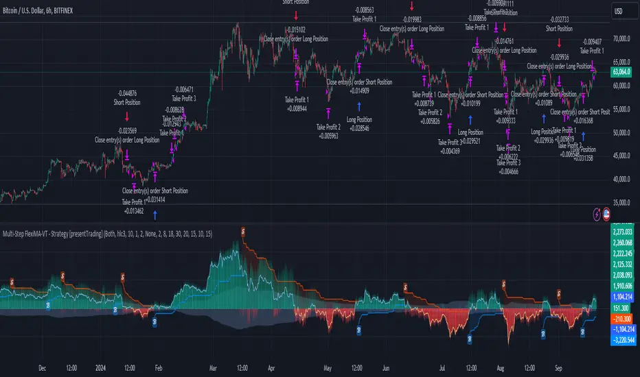
Multi-Step FlexiMA - Strategy [presentTrading]It's time to come back! hope I can not to be busy for a while.
█ Introduction and How It Is Different
The FlexiMA Variance Tracker is a unique trading strategy that calculates a series of deviations between the price (or another indicator source) and a variable-length moving average (MA). Unlike traditional strategies that use fixed-length moving averages, the length of the MA in this system varies within a defined range. The length changes dynamically based on a starting factor and an increment factor, creating a more adaptive approach to market conditions.
This strategy integrates Multi-Step Take Profit (TP) levels, allowing for partial exits at predefined price increments. It enables traders to secure profits at different stages of a trend, making it ideal for volatile markets where taking full profits at once might lead to missed opportunities if the trend continues.
BTCUSD 6hr Performance
█ Strategy, How It Works: Detailed Explanation
🔶 FlexiMA Concept
The FlexiMA (Flexible Moving Average) is at the heart of this strategy. Unlike traditional MA-based strategies where the MA length is fixed (e.g., a 50-period SMA), the FlexiMA varies its length with each iteration. This is done using a **starting factor** and an **increment factor**.
The formula for the moving average length at each iteration \(i\) is:
`MA_length_i = indicator_length * (starting_factor + i * increment_factor)`
Where:
- `indicator_length` is the user-defined base length.
- `starting_factor` is the initial multiplier of the base length.
- `increment_factor` increases the multiplier in each iteration.
Each iteration applies a **simple moving average** (SMA) to the chosen **indicator source** (e.g., HLC3) with a different length based on the above formula. The deviation between the current price and the moving average is then calculated as follows:
`deviation_i = price_current - MA_i`
These deviations are normalized using one of the following methods:
- **Max-Min normalization**:
`normalized_i = (deviation_i - min(deviations)) / range(deviations)`
- **Absolute Sum normalization**:
`normalized_i = deviation_i / sum(|deviation_i|)`
The **median** and **standard deviation (stdev)** of the normalized deviations are then calculated as follows:
`median = median(normalized deviations)`
For the standard deviation:
`stdev = sqrt((1/(N-1)) * sum((normalized_i - mean)^2))`
These values are plotted to provide a clear indication of how the price is deviating from its variable-length moving averages.
For more detail:
🔶 Multi-Step Take Profit
This strategy uses a multi-step take profit system, allowing for exits at different stages of a trade based on the percentage of price movement. Three take-profit levels are defined:
- Take Profit Level 1 (TP1): A small, quick profit level (e.g., 2%).
- Take Profit Level 2 (TP2): A medium-level profit target (e.g., 8%).
- Take Profit Level 3 (TP3): A larger, more ambitious target (e.g., 18%).
At each level, a corresponding percentage of the trade is exited:
- TP Percent 1: E.g., 30% of the position.
- TP Percent 2: E.g., 20% of the position.
- TP Percent 3: E.g., 15% of the position.
This approach ensures that profits are locked in progressively, reducing the risk of market reversals wiping out potential gains.
Local
🔶 Trade Entry and Exit Conditions
The entry and exit signals are determined by the interaction between the **SuperTrend Polyfactor Oscillator** and the **median** value of the normalized deviations:
- Long entry: The SuperTrend turns bearish, and the median value of the deviations is positive.
- Short entry: The SuperTrend turns bullish, and the median value is negative.
Similarly, trades are exited when the SuperTrend flips direction.
* The SuperTrend Toolkit is made by @EliCobra
█ Trade Direction
The strategy allows users to specify the desired trade direction:
- Long: Only long positions will be taken.
- Short: Only short positions will be taken.
- Both: Both long and short positions are allowed based on the conditions.
This flexibility allows the strategy to adapt to different market conditions and trading styles, whether you're looking to buy low and sell high, or sell high and buy low.
█ Usage
This strategy can be applied across various asset classes, including stocks, cryptocurrencies, and forex. The primary use case is to take advantage of market volatility by using a flexible moving average and multiple take-profit levels to capture profits incrementally as the market moves in your favor.
How to Use:
1. Configure the Inputs: Start by adjusting the **Indicator Length**, **Starting Factor**, and **Increment Factor** to suit your chosen asset. The defaults work well for most markets, but fine-tuning them can improve performance.
2. Set the Take Profit Levels: Adjust the three **TP levels** and their corresponding **percentages** based on your risk tolerance and the expected volatility of the market.
3. Monitor the Strategy: The SuperTrend and the FlexiMA variance tracker will provide entry and exit signals, automatically managing the positions and taking profits at the pre-set levels.
█ Default Settings
The default settings for the strategy are configured to provide a balanced approach that works across different market conditions:
Indicator Length (10):
This controls the base length for the moving average. A lower length makes the moving average more responsive to price changes, while a higher length smooths out fluctuations, making the strategy less sensitive to short-term price movements.
Starting Factor (1.0):
This determines the initial multiplier applied to the moving average length. A higher starting factor will increase the average length, making it slower to react to price changes.
Increment Factor (1.0):
This increases the moving average length in each iteration. A larger increment factor creates a wider range of moving average lengths, allowing the strategy to track both short-term and long-term trends simultaneously.
Normalization Method ('None'):
Three methods of normalization can be applied to the deviations:
- None: No normalization applied, using raw deviations.
- Max-Min: Normalizes based on the range between the maximum and minimum deviations.
- Absolute Sum: Normalizes based on the total sum of absolute deviations.
Take Profit Levels:
- TP1 (2%): A quick exit to capture small price movements.
- TP2 (8%): A medium-term profit target for stronger trends.
- TP3 (18%): A long-term target for strong price moves.
Take Profit Percentages:
- TP Percent 1 (30%): Exits 30% of the position at TP1.
- TP Percent 2 (20%): Exits 20% of the position at TP2.
- TP Percent 3 (15%): Exits 15% of the position at TP3.
Effect of Variables on Performance:
- Short Indicator Lengths: More responsive to price changes but prone to false signals.
- Higher Starting Factor: Slows down the response, useful for longer-term trend following.
- Higher Increment Factor: Widens the variability in moving average lengths, making the strategy adapt to both short-term and long-term price trends.
- Aggressive Take Profit Levels: Allows for quick profit-taking in volatile markets but may exit positions prematurely in strong trends.
The default configuration offers a moderate balance between short-term responsiveness and long-term trend capturing, suitable for most traders. However, users can adjust these variables to optimize performance based on market conditions and personal preferences.
QuantBuilder | FractalystWhat's the strategy's purpose and functionality?
QuantBuilder is designed for both traders and investors who want to utilize mathematical techniques to develop profitable strategies through backtesting on historical data.
The primary goal is to develop profitable quantitive strategies that not only outperform the underlying asset in terms of returns but also minimize drawdown.
For instance, consider Bitcoin (BTC), which has experienced significant volatility, averaging an estimated 200% annual return over the past decade, with maximum drawdowns exceeding -80%. By employing this strategy with diverse entry and exit techniques, users can potentially seek to enhance their Compound Annual Growth Rate (CAGR) while managing risk to maintain a lower maximum drawdown.
While this strategy employs quantitative techniques, including mathematical methods such as probabilities and positive expected values, it demonstrates exceptional efficacy across all markets. It particularly excels in futures, indices, stocks, cryptocurrencies, and commodities, leveraging their inherent trending behaviors for optimized performance.
In both trending and consolidating market conditions, QuantBuilder employs a combination of multi-timeframe probabilities, expected values, directional biases, moving averages and diverse entry models to identify and capitalize on bullish market movements.
How does the strategy perform for both investors and traders?
The strategy has two main modes, tailored for different market participants: Traders and Investors.
1. Trading:
- Designed for traders looking to capitalize on bullish markets.
- Utilizes a percentage risk per trade to manage risk and optimize returns.
- Suitable for both swing and intraday trading with a focus on probabilities and risk per trade approach.
2. Investing:
- Geared towards investors who aim to capitalize on bullish trending markets without using leverage while mitigating the asset's maximum drawdown.
- Utilizes pre-define percentage of the equity to buy, hold, and manage the asset.
- Focuses on long-term growth and capital appreciation by fully/partially investing in the asset during bullish conditions.
How does the strategy identify market structure? What are the underlying calculations?
The strategy utilizes an efficient logic with for loops to pinpoint the first swing candle featuring a pivot of 2, establishing the point at which the break of structure begins.
What entry criteria are used in this script? What are the underlying calculations?
The script utilizes two entry models: BreakOut and fractal.
Underlying Calculations:
Breakout: The script assigns the most recent swing high to a variable. When the price closes above this level and all other conditions are met, the script executes a breakout entry (conservative approach).
Fractal: The script identifies a swing low with a period of 2. Once this condition is met, the script executes the trade (aggressive approach).
How does the script calculate probabilities? What are the underlying calculations?
The script calculates probabilities by monitoring price interactions with liquidity levels. Here’s how the underlying calculations work:
Tracking Price Hits: The script counts the number of times the price taps into each liquidity side after the EQM level is activated. This data is stored in an array for further analysis.
Sample Size Consideration: The total number of price interactions serves as the sample size for calculating probabilities.
Probability Calculation: For each liquidity side, the script calculates the probability by taking the average of the recorded hits. This allows for a dynamic assessment of the likelihood that a particular side will be hit next, based on historical performance.
Dynamic Adjustment: As new price data comes in, the probabilities are recalculated, providing real-time aduptive insights into market behavior.
Note: The calculations are performed independently for each directional range. A range is considered bearish if the previous breakout was through a sellside liquidity. Conversely, a range is considered bullish if the most recent breakout was through a buyside liquidity.
How does the script calculate expected values? What are the underlying calculations?
The script calculates expected values by leveraging the probabilities of winning and losing trades, along with their respective returns. The process involves the following steps:
This quantitative methodology provides a robust framework for assessing the expected performance of trading strategies based on historical data and backtesting results.
How is the contextual bias calculated? What are the underlying calculations?
The contextual bias in the QuantBuilder script is calculated through a structured approach that assesses market structure based on swing highs and lows. Here’s how it works:
Identification of Swing Points: The script identifies significant swing points using a defined pivot logic, focusing on the first swing high and swing low. This helps establish critical levels for determining market structure.
Break of Structure (BOS) Assessment:
Bullish BOS: The script recognizes a bullish break of structure when a candle closes above the first swing high, followed by at least one swing low.
Bearish BOS: Conversely, a bearish break of structure is identified when a candle closes below the first swing low, followed by at least one swing high.
Bias Assignment: Based on the identified break of structure, the script assigns directional biases:
A bullish bias is assigned if a bullish BOS is confirmed.
A bearish bias is assigned if a bearish BOS is confirmed.
Quantitative Evaluation: Each identified bias is quantitatively evaluated, allowing the script to assign numerical values representing the strength of each bias. This quantification aids in assessing the reliability of market sentiment across multiple timeframes.
What's the purpose of using moving averages in this strategy? What are the underlying calculations?
Using moving averages is a widely-used technique to trade with the trend.
The main purpose of using moving averages in this strategy is to filter out bearish price action and to only take trades when the price is trading ABOVE specified moving averages.
The script uses different types of moving averages with user-adjustable timeframes and periods/lengths, allowing traders to try out different variations to maximize strategy performance and minimize drawdowns.
By applying these calculations, the strategy effectively identifies bullish trends and avoids market conditions that are not conducive to profitable trades.
The MA filter allows traders to choose whether they want a specific moving average above or below another one as their entry condition.
What type of stop-loss identification method are used in this strategy? What are the underlying calculations?
- Initial Stop-loss:
1. ATR Based:
The Average True Range (ATR) is a method used in technical analysis to measure volatility. It is not used to indicate the direction of price but to measure volatility, especially volatility caused by price gaps or limit moves.
Calculation:
- To calculate the ATR, the True Range (TR) first needs to be identified. The TR takes into account the most current period high/low range as well as the previous period close.
The True Range is the largest of the following:
- Current Period High minus Current Period Low
- Absolute Value of Current Period High minus Previous Period Close
- Absolute Value of Current Period Low minus Previous Period Close
- The ATR is then calculated as the moving average of the TR over a specified period. (The default period is 14)
2. ADR Based:
The Average Day Range (ADR) is an indicator that measures the volatility of an asset by showing the average movement of the price between the high and the low over the last several days.
Calculation:
- To calculate the ADR for a particular day:
- Calculate the average of the high prices over a specified number of days.
- Calculate the average of the low prices over the same number of days.
- Find the difference between these average values.
- The default period for calculating the ADR is 14 days. A shorter period may introduce more noise, while a longer period may be slower to react to new market movements.
3. PL Based:
This method places the stop-loss at the low of the previous candle.
If the current entry is based on the hunt entry strategy, the stop-loss will be placed at the low of the candle that wicks through the lower FRMA band.
Example:
If the previous candle's low is 100, then the stop-loss will be set at 100.
This method ensures the stop-loss is placed just below the most recent significant low, providing a logical and immediate level for risk management.
- Trailing Stop-Loss:
One of the key elements of this strategy is its ability to detect structural liquidity and structural invalidation levels across multiple timeframes to trail the stop-loss once the trade is in running profits.
By utilizing this approach, the strategy allows enough room for price to run.
By using these methods, the strategy dynamically adjusts the initial stop-loss based on market volatility, helping to protect against adverse price movements while allowing for enough room for trades to develop.
Each market behaves differently across various timeframes, and it is essential to test different parameters and optimizations to find out which trailing stop-loss method gives you the desired results and performance.
What type of break-even and take profit identification methods are used in this strategy? What are the underlying calculations?
For Break-Even:
Percentage (%) Based:
Moves the initial stop-loss to the entry price when the price reaches a certain percentage above the entry.
Calculation:
Break-even level = Entry Price * (1 + Percentage / 100)
Example:
If the entry price is $100 and the break-even percentage is 5%, the break-even level is $100 * 1.05 = $105.
Risk-to-Reward (RR) Based:
Moves the initial stop-loss to the entry price when the price reaches a certain RR ratio.
Calculation:
Break-even level = Entry Price + (Initial Risk * RR Ratio)
For TP1 (Take Profit 1):
- You can choose to set a take profit level at which your position gets fully closed or 50% if the TP2 boolean is enabled.
- Similar to break-even, you can select either a percentage (%) or risk-to-reward (RR) based take profit level, allowing you to set your TP1 level as a percentage amount above the entry price or based on RR.
For TP2 (Take Profit 2):
- You can choose to set a take profit level at which your position gets fully closed.
- As with break-even and TP1, you can select either a percentage (%) or risk-to-reward (RR) based take profit level, allowing you to set your TP2 level as a percentage amount above the entry price or based on RR.
What's the day filter Filter, what does it do?
The day filter allows users to customize the session time and choose the specific days they want to include in the strategy session. This helps traders tailor their strategies to particular trading sessions or days of the week when they believe the market conditions are more favorable for their trading style.
Customize Session Time:
Users can define the start and end times for the trading session.
This allows the strategy to only consider trades within the specified time window, focusing on periods of higher market activity or preferred trading hours.
Select Days:
Users can select which days of the week to include in the strategy.
This feature is useful for excluding days with historically lower volatility or unfavorable trading conditions (e.g., Mondays or Fridays).
Benefits:
Focus on Optimal Trading Periods:
By customizing session times and days, traders can focus on periods when the market is more likely to present profitable opportunities.
Avoid Unfavorable Conditions:
Excluding specific days or times can help avoid trading during periods of low liquidity or high unpredictability, such as major news events or holidays.
What tables are available in this script?
- Summary: Provides a general overview, displaying key performance parameters such as Net Profit, Profit Factor, Max Drawdown, Average Trade, Closed Trades and more.
Total Commission: Displays the cumulative commissions incurred from all trades executed within the selected backtesting window. This value is derived by summing the commission fees for each trade on your chart.
Average Commission: Represents the average commission per trade, calculated by dividing the Total Commission by the total number of closed trades. This metric is crucial for assessing the impact of trading costs on overall profitability.
Avg Trade: The sum of money gained or lost by the average trade generated by a strategy. Calculated by dividing the Net Profit by the overall number of closed trades. An important value since it must be large enough to cover the commission and slippage costs of trading the strategy and still bring a profit.
MaxDD: Displays the largest drawdown of losses, i.e., the maximum possible loss that the strategy could have incurred among all of the trades it has made. This value is calculated separately for every bar that the strategy spends with an open position.
Profit Factor: The amount of money a trading strategy made for every unit of money it lost (in the selected currency). This value is calculated by dividing gross profits by gross losses.
Avg RR: This is calculated by dividing the average winning trade by the average losing trade. This field is not a very meaningful value by itself because it does not take into account the ratio of the number of winning vs losing trades, and strategies can have different approaches to profitability. A strategy may trade at every possibility in order to capture many small profits, yet have an average losing trade greater than the average winning trade. The higher this value is, the better, but it should be considered together with the percentage of winning trades and the net profit.
Winrate: The percentage of winning trades generated by a strategy. Calculated by dividing the number of winning trades by the total number of closed trades generated by a strategy. Percent profitable is not a very reliable measure by itself. A strategy could have many small winning trades, making the percent profitable high with a small average winning trade, or a few big winning trades accounting for a low percent profitable and a big average winning trade. Most mean-reversion successful strategies have a percent profitability of 40-80% but are profitable due to risk management control.
BE Trades: Number of break-even trades, excluding commission/slippage.
Losing Trades: The total number of losing trades generated by the strategy.
Winning Trades: The total number of winning trades generated by the strategy.
Total Trades: Total number of taken traders visible your charts.
Net Profit: The overall profit or loss (in the selected currency) achieved by the trading strategy in the test period. The value is the sum of all values from the Profit column (on the List of Trades tab), taking into account the sign.
- Monthly: Displays performance data on a month-by-month basis, allowing users to analyze performance trends over each month and year.
- Weekly: Displays performance data on a week-by-week basis, helping users to understand weekly performance variations.
- UI Table: A user-friendly table that allows users to view and save the selected strategy parameters from user inputs. This table enables easy access to key settings and configurations, providing a straightforward solution for saving strategy parameters by simply taking a screenshot with Alt + S or ⌥ + S.
User-input styles and customizations:
To facilitate studying historical data, all conditions and filters can be applied to your charts. By plotting background colors on your charts, you'll be able to identify what worked and what didn't in certain market conditions.
Please note that all background colors in the style are disabled by default to enhance visualization.
How to Use This Quantitive Strategy Builder to Create a Profitable Edge and System?
Choose Your Strategy mode:
- Decide whether you are creating an investing strategy or a trading strategy.
Select a Market:
- Choose a one-sided market such as stocks, indices, or cryptocurrencies.
Historical Data:
- Ensure the historical data covers at least 10 years of price action for robust backtesting.
Timeframe Selection:
- Choose the timeframe you are comfortable trading with. It is strongly recommended to use a timeframe above 15 minutes to minimize the impact of commissions/slippage on your profits.
Set Commission and Slippage:
- Properly set the commission and slippage in the strategy properties according to your broker/prop firm specifications.
Parameter Optimization:
- Use trial and error to test different parameters until you find the performance results you are looking for in the summary table or, preferably, through deep backtesting using the strategy tester.
Trade Count:
- Ensure the number of trades is 200 or more; the higher, the better for statistical significance.
Positive Average Trade:
- Make sure the average trade is above zero.
(An important value since it must be large enough to cover the commission and slippage costs of trading the strategy and still bring a profit.)
Performance Metrics:
- Look for a high profit factor, and net profit with minimum drawdown.
- Ideally, aim for a drawdown under 20-30%, depending on your risk tolerance.
Refinement and Optimization:
- Try out different markets and timeframes.
- Continue working on refining your edge using the available filters and components to further optimize your strategy.
What makes this strategy original?
QuantBuilder stands out due to its unique combination of quantitative techniques and innovative algorithms that leverage historical data for real-time trading decisions. Unlike most algorithmic strategies that work based on predefined rules, this strategy adapts to real-time market probabilities and expected values, enhancing its reliability. Key features include:
Mathematical Framework: The strategy integrates advanced mathematical concepts, such as probabilities and expected values, to assess trade viability and optimize decision-making.
Multi-Timeframe Analysis: By utilizing multi-timeframe probabilities, QuantBuilder provides a comprehensive view of market conditions, enhancing the accuracy of entry and exit points.
Dynamic Market Structure Identification: The script employs a systematic approach to identify market structure changes, utilizing a blend of swing highs and lows to detect contextual/direction bias of the market.
Built-in Trailing Stop Loss: The strategy features a dynamic trailing stop loss based on multi-timeframe analysis of market structure. This allows traders to lock in profits while adapting to changing market conditions, ensuring that exits are executed at optimal levels without prematurely closing positions.
Robust Performance Metrics: With detailed performance tables and visualizations, users can easily evaluate strategy effectiveness and adjust parameters based on historical performance.
Adaptability: The strategy is designed to work across various markets and timeframes, making it versatile for different trading styles and objectives.
Suitability for Investors and Traders: QuantBuilder is ideal for both investors and traders looking to rely on mathematically proven data to create profitable strategies, ensuring that decisions are grounded in quantitative analysis.
These original elements combine to create a powerful tool that can help both traders and investors to build and refine profitable strategies based on algorithmic quantitative analysis.
Terms and Conditions | Disclaimer
Our charting tools are provided for informational and educational purposes only and should not be construed as financial, investment, or trading advice. They are not intended to forecast market movements or offer specific recommendations. Users should understand that past performance does not guarantee future results and should not base financial decisions solely on historical data.
Built-in components, features, and functionalities of our charting tools are the intellectual property of @Fractalyst Unauthorized use, reproduction, or distribution of these proprietary elements is prohibited.
By continuing to use our charting tools, the user acknowledges and accepts the Terms and Conditions outlined in this legal disclaimer and agrees to respect our intellectual property rights and comply with all applicable laws and regulations.

Larry Conners Vix Reversal II Strategy (approx.)This Pine Script™ strategy is a modified version of the original Larry Connors VIX Reversal II Strategy, designed for short-term trading in market indices like the S&P 500. The strategy utilizes the Relative Strength Index (RSI) of the VIX (Volatility Index) to identify potential overbought or oversold market conditions. The logic is based on the assumption that extreme levels of market volatility often precede reversals in price.
How the Strategy Works
The strategy calculates the RSI of the VIX using a 25-period lookback window. The RSI is a momentum oscillator that measures the speed and change of price movements. It ranges from 0 to 100 and is often used to identify overbought and oversold conditions in assets.
Overbought Signal: When the RSI of the VIX rises above 61, it signals a potential overbought condition in the market. The strategy looks for a RSI downtick (i.e., when RSI starts to fall after reaching this level) as a trigger to enter a long position.
Oversold Signal: Conversely, when the RSI of the VIX drops below 42, the market is considered oversold. A RSI uptick (i.e., when RSI starts to rise after hitting this level) serves as a signal to enter a short position.
The strategy holds the position for a minimum of 7 days and a maximum of 12 days, after which it exits automatically.
Larry Connors: Background
Larry Connors is a prominent figure in quantitative trading, specializing in short-term market strategies. He is the co-author of several influential books on trading, such as Street Smarts (1995), co-written with Linda Raschke, and How Markets Really Work. Connors' work focuses on developing rules-based systems using volatility indicators like the VIX and oscillators such as RSI to exploit mean-reversion patterns in financial markets.
Risks of the Strategy
While the Larry Connors VIX Reversal II Strategy can capture reversals in volatile market environments, it also carries significant risks:
Over-Optimization: This modified version adjusts RSI levels and holding periods to fit recent market data. If market conditions change, the strategy might no longer be effective, leading to false signals.
Drawdowns in Trending Markets: This is a mean-reversion strategy, designed to profit when markets return to a previous mean. However, in strongly trending markets, especially during extended bull or bear phases, the strategy might generate losses due to early entries or exits.
Volatility Risk: Since this strategy is linked to the VIX, an instrument that reflects market volatility, large spikes in volatility can lead to unexpected, fast-moving market conditions, potentially leading to larger-than-expected losses.
Scientific Literature and Supporting Research
The use of RSI and VIX in trading strategies has been widely discussed in academic research. RSI is one of the most studied momentum oscillators, and numerous studies show that it can capture mean-reversion effects in various markets, including equities and derivatives.
Wong et al. (2003) investigated the effectiveness of technical trading rules such as RSI, finding that it has predictive power in certain market conditions, particularly in mean-reverting markets .
The VIX, often referred to as the “fear index,” reflects market expectations of volatility and has been a focal point in research exploring volatility-based strategies. Whaley (2000) extensively reviewed the predictive power of VIX, noting that extreme VIX readings often correlate with turning points in the stock market .
Modified Version of Original Strategy
This script is a modified version of Larry Connors' original VIX Reversal II strategy. The key differences include:
Adjusted RSI period to 25 (instead of 2 or 4 commonly used in Connors’ other work).
Overbought and oversold levels modified to 61 and 42, respectively.
Specific holding period (7 to 12 days) is predefined to reduce holding risk.
These modifications aim to adapt the strategy to different market environments, potentially enhancing performance under specific volatility conditions. However, as with any system, constant evaluation and testing in live markets are crucial.
References
Wong, W. K., Manzur, M., & Chew, B. K. (2003). How rewarding is technical analysis? Evidence from Singapore stock market. Applied Financial Economics, 13(7), 543-551.
Whaley, R. E. (2000). The investor fear gauge. Journal of Portfolio Management, 26(3), 12-17.
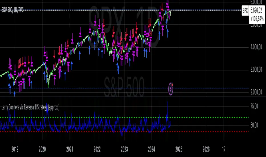
Nifty scalping 3 minutes options on Dhan
Strategy Description for Publishing: Nifty Scalping 3 Minutes Options on Dhan
Overview:
The Nifty Scalping 3 Minutes Options on Dhan strategy is an enhanced version tailored for trading Nifty Options, building on the core logic used in the previously published Nifty Scalping 3 Minutes Strategy. This strategy provides automated order execution via JSON alerts for seamless integration with the Dhan platform, enabling hands-free options trading.
This system is designed to capture short-term market moves using a combination of technical indicators like the Jurik Moving Average (JMA), Exponential Moving Average (EMA), and Bollinger Bands, while also allowing traders to manage risk effectively with custom inputs for maximum loss per lot and partial profit booking.
For more details on the core logic and performance of the strategy, please refer to our earlier published strategy:
Nifty Scalping 3 Minutes Strategy
Key Features:
JMA and EMA Crossovers: Trades are executed when the Jurik Moving Average (JMA) crosses over (for long trades) or under (for short trades) the Exponential Moving Average (EMA), signaling trend direction.
Price-Volume Spike Detection: Ensures that trades are executed only when significant market activity is detected, avoiding low-momentum conditions. Price-volume relationships are monitored to confirm the strength of market movements.
Bollinger Band Noise Filter: Filters out low-volatility periods by executing trades only when prices break through the upper or lower Bollinger Bands, confirming high volatility.
Customizable Risk Management: Traders can set their own maximum risk per lot (e.g., ₹650), and the strategy adjusts the stop-loss accordingly to ensure that no trade exceeds this threshold.
Partial Profit Booking: A predefined percentage (e.g., 60%) of the position can be booked as profit once the first profit target is reached, with the remaining position trailed using an ATR-based stop.
STBT/BTST Support: The strategy offers the flexibility to carry trades overnight, supporting Sell Today, Buy Tomorrow (STBT) and Buy Today, Sell Tomorrow (BTST).
Time-Based Exit: The strategy automatically closes any open positions by 3:20 PM to avoid the volatile end-of-day market conditions.
Inputs for Traders:
Option Quantity: Select the number of contracts to trade (e.g., 10).
Maximum Risk Per Lot: Set your maximum allowable loss per lot (e.g., ₹650), ensuring that your risk is managed effectively.
Partial Profit Booking Percentage: Define what percentage of your position to book as profit (e.g., 60%) when the first target is hit.
STBT/BTST Option: Choose whether to allow positions to be carried overnight.
Alert Secret Key: Input your secret key for the Dhan platform to trigger automated orders via JSON alerts.
Option Expiry Date: Specify the expiry date for the options being traded.
Trade Logic:
Long Trades: Triggered when JMA crosses above EMA, supported by filters like price-volume spikes and Bollinger Band breakouts. The strategy waits for momentum confirmation before entering long trades, with stop-loss and profit-taking mechanisms in place.
Short Trades: Triggered when JMA crosses below EMA, with confirmation through additional filters to ensure strong market trends before entering short positions.
Risk Management:
Stop-Loss: A dynamic stop-loss is placed for each trade based on the trader's maximum risk per lot. The stop-loss adapts to market conditions using ATR trailing stops to capture further gains as the trade progresses.
Partial Profit Booking: Once the first profit target is hit (2.1x risk for long trades and 2.5x risk for short trades), a percentage of the position is booked as profit, and the remainder is trailed using an ATR stop.
Automation via JSON Alerts:This strategy sends automated JSON alerts to the Dhan platform for seamless execution of orders. The alerts support multi-leg orders for both entry and exit, ensuring that trades are executed efficiently without manual intervention.
Why Use This Strategy?
The Nifty Scalping 3 Minutes Options on Dhan strategy is perfect for traders who want to capitalize on quick market moves in options, backed by strong risk management and automation. With automated alerts, customizable inputs, and advanced technical filters, this strategy is ideal for traders looking to engage in high-probability options trades with minimal effort.
For more detailed information about the underlying logic, you can refer to the previously published Nifty Scalping 3 Minutes Strategy here.
Disclaimer:
This strategy is provided as an educational tool, and we are not affiliated with or sponsored by Dhan. The strategy integrates with the Dhan platform for automated trading, but there is no formal relationship between this strategy and Dhan.

Nifty scalping 3 minutesOverview:
The "Nifty Scalping 3 Minutes" strategy is a uniquely tailored trading system for Nifty Futures traders, with a clear focus on capital preservation, dynamic risk management, and high-probability trade entries. This strategy uses unique combination of standard technical indicators like Jurik Moving Average (JMA), Exponential Moving Average (EMA), and Bollinger Bands, but it truly stands out through its Price-Volume Spike Detection system—a unique mechanism designed to trigger trades only during periods of high momentum and market participation. The strategy also incorporates robust risk management, ensuring that traders minimize losses while maximizing profits. in complete back test range max drawdown is less than 1%
Scalping Approach and Requirements:
The strategy focuses on quick in and out trades, aiming to capture small, quick profits during periods of heightened market activity. For optimal performance, traders should have ₹2,00,000 or more in capital available per trade. The dynamic lot calculation and risk controls require this level of capital to function effectively.
Small, frequent trades are the focus, and the strategy is ideal for traders comfortable with high-frequency executions. Traders with insufficient capital or those not comfortable with frequent trades may find this strategy unsuitable.
Default Properties for Publication:
Initial Capital: ₹2,000,000
Lot Size: 25 contracts (adjusted dynamically based on available margin)
Stop-Loss: Risk per trade capped at 1% of equity.
Slippage and Commission: Realistic values are factored into the backtesting.
Key Feature: Price-Volume Spike Detection
1. Condition: Trades are executed only when there is a significant price spike confirmed by a volume spike. The candle width is calculated by multiplying the price change (difference between the candle's open and close) by the volume, and this result is compared to a 126-period average of both price and volume.
A trade is triggered when the current price-volume spike exceeds this average by a preset volume multiplier (default set at 3). This ensures that both the price change and volume are unusually strong compared to normal market behavior.
2. Reasoning: Many traders fail to incorporate the relationship between price movement and volume effectively. By using this Price-Volume Spike Detection mechanism, the strategy ensures that it only enters trades during periods of strong market momentum when both price and volume confirm a real market move, not just noise or small fluctuations.
The 126-period moving average of volume is chosen specifically because it represents a complete trading session on the 3-minute chart. This ensures that the volume spike is compared against a realistic baseline of daily activity, making the detection more robust and reliable.
The volume multiplier allows flexibility in determining the threshold for a significant spike, enabling users to fine-tune the strategy according to their risk tolerance and market conditions.
Trade Placement Logic:
1. Trend Confirmation with JMA and EMA:
Condition: The strategy will only consider entering a trade when JMA crosses above EMA for a long trade or JMA crosses below EMA for a short trade.
Reasoning: The JMA is used for its low lag and responsiveness, allowing it to capture early trends, while the EMA adds a level of confirmation by weighing recent price action more heavily. This dual confirmation ensures that trades are entered only when a solid trend is in place.
2. Bollinger Bands for Volatility Breakouts:
Condition: In addition to the JMA-EMA crossover, the price must break outside the Bollinger Bands—above the upper band for long trades, or below the lower band for short trades.
Reasoning: Bollinger Bands are a volatility indicator. By requiring a price breakout beyond the bands, the strategy ensures that trades are placed during periods of high volatility, avoiding low-momentum, sideways markets.
3. Volume and Price Confirmation (Price-Volume Spike Detection):
Condition: A trade is only triggered if the price-volume spike condition is met. This ensures that the market move is backed by strong volume and that the price change is significant relative to the recent average activity.
Reasoning: This condition filters out low-volume environments where price movements are more likely to reverse or stall. By waiting for a spike in both price and volume, the strategy ensures that it enters trades during high-momentum periods, where follow-through is more likely.
Exit Logic and Risk Management:
1. Stop-Loss (SL) Placement:
Condition: Upon entering a trade, an initial stop-loss is placed below the candle low for long trades or above the candle high for short trades. This is adjusted if the risk exceeds 1% of total capital.
Reasoning: The stop-loss is placed at a logical level that accounts for recent price action, ensuring that the trade is given room to develop while protecting capital from unexpected market reversals.
2. Profit Target and Partial Profit Booking:
Condition: The first profit target is set at 2.1x the initial risk for long trades, and 2.5x the initial risk for short trades.
Reasoning: The 2.1x risk-reward ratio for long trades provides a solid return while maintaining a conservative risk profile. For short trades, the strategy uses a higher 2.5x risk-reward ratio because market falls tend to be sharper and quicker than rises, allowing for larger profit targets to be reached more reliably.
Partial Profit Booking: Once the first target is hit, 60% of the position is closed to lock in profits. The remaining 40% is left to run with a trailing stop.
3. ATR-Based Trailing Stop:
Condition: Once the first target is hit, the ATR (Average True Range) trailing stop is applied to the remaining position. This dynamically adjusts the stop-loss as the trade moves in a favorable direction.
Reasoning: The trailing stop allows the trade to capture further gains if the trend continues, while protecting profits if the momentum weakens. The ATR ensures that the stop adjusts according to the market's current volatility, providing flexibility and protection.
4. Time-Based Exit:
Condition: If a trade is still open by 3:20 PM, it is automatically closed to avoid end-of-day volatility.
Reasoning: The time-based exit ensures that trades are not held into the often-volatile closing minutes of the market, reducing the risk of unexpected price swings.
Capital and Risk Management:
1. Lot Size Calculation:
Condition: The strategy calculates the number of lots dynamically based on the available margin. It uses only 10% of total equity for each trade, and ensures that the maximum risk per trade does not exceed 1% of total capital.
Reasoning: This ensures that traders are not over-leveraged and that the risk is controlled for each trade. Capital protection is at the core of the strategy, ensuring that even during adverse market conditions, the trader’s capital is preserved.
2. Stop-Loss Protection:
Condition: The stop-loss is designed to ensure that no more than 1% of capital is at risk in any trade.
Reasoning: By limiting risk exposure, the strategy focuses on long-term capital preservation while still allowing for profitable trades in favorable market conditions.
STBT/BTST Facilitation:
1. Feature: The strategy allows traders the option to hold positions overnight, facilitating STBT (Sell Today Buy Tomorrow) and BTST (Buy Today Sell Tomorrow) trades.
Reasoning: Backtests show that holding positions overnight when all trade conditions are still valid can lead to beneficial outcomes. This feature allows traders to take advantage of overnight market movements, providing flexibility beyond intraday trades.
Why This Strategy Stands Out:
Price-Volume Spike Detection: Unlike traditional strategies, this one uniquely focuses on Price-Volume Spike Detection to filter out low-probability trades. By ensuring that both price and volume spikes are present, the strategy guarantees that trades are placed only when there is significant market momentum.
Risk Management with Capital Protection: The strategy strictly limits the risk per trade to 1% of capital, ensuring long-term capital preservation. This is especially important for traders who wish to avoid large drawdowns and prefer a sustainable approach to trading.
2.5x Risk-Reward for Short Trades: Recognizing the sharpness of market declines, the strategy employs a 2.5x risk-reward ratio for short trades, maximizing profits during bearish trends.
Dynamic Exit Strategy: With partial profit booking and ATR-based trailing stops, the strategy is designed to capture gains efficiently while protecting capital through dynamic exit conditions.
Summary of Execution:
Entry: Triggered when JMA crosses EMA, combined with Bollinger Band breakouts and Price-Volume Spike Detection.
Capital Management: Trades are executed with 10% of available capital, and the risk per trade is capped at 1%.
Exit: Trades exit when stop-loss, ATR trailing stop, or time-based exit conditions are met.
Profit Booking: 60% of the position is closed at the first target, with the remainder trailed using an ATR-based stop.

BTC 5 min SHBHilalimSB A Wedding Gift 🌙
What is HilalimSB🌙?
First of all, as mentioned in the title, HilalimSB is a wedding gift.
HilalimSB - Revealing the Secrets of the Trend
HilalimSB is a powerful indicator designed to help investors analyze market trends and optimize trading strategies. Designed to uncover the secrets at the heart of the trend, HilalimSB stands out with its unique features and impressive algorithm.
Hilalim Algorithm and Fixed ATR Value:
HilalimSB is equipped with a special algorithm called "Hilalim" to detect market trends. This algorithm can delve into the depths of price movements to determine the direction of the trend and provide users with the ability to predict future price movements. Additionally, HilalimSB uses its own fixed Average True Range (ATR) value. ATR is an indicator that measures price movement volatility and is often used to determine the strength of a trend. The fixed ATR value of HilalimSB has been tested over long periods and its reliability has been proven. This allows users to interpret the signals provided by the indicator more reliably.
ATR Calculation Steps
1.True Range Calculation:
+ The True Range (TR) is the greatest of the following three values:
1. Current high minus current low
2. Current high minus previous close (absolute value)
3. Current low minus previous close (absolute value)
2.Average True Range (ATR) Calculation:
-The initial ATR value is calculated as the average of the TR values over a specified period
(typically 14 periods).
-For subsequent periods, the ATR is calculated using the following formula:
ATRt=(ATRt−1×(n−1)+TRt)/n
Where:
+ ATRt is the ATR for the current period,
+ ATRt−1 is the ATR for the previous period,
+ TRt is the True Range for the current period,
+ n is the number of periods.
Pine Script to Calculate ATR with User-Defined Length and Multiplier
Here is the Pine Script code for calculating the ATR with user-defined X length and Y multiplier:
//@version=5
indicator("Custom ATR", overlay=false)
// User-defined inputs
X = input.int(14, minval=1, title="ATR Period (X)")
Y = input.float(1.0, title="ATR Multiplier (Y)")
// True Range calculation
TR1 = high - low
TR2 = math.abs(high - close )
TR3 = math.abs(low - close )
TR = math.max(TR1, math.max(TR2, TR3))
// ATR calculation
ATR = ta.rma(TR, X)
// Apply multiplier
customATR = ATR * Y
// Plot the ATR value
plot(customATR, title="Custom ATR", color=color.blue, linewidth=2)
This code can be added as a new Pine Script indicator in TradingView, allowing users to calculate and display the ATR on the chart according to their specified parameters.
HilalimSB's Distinction from Other ATR Indicators
HilalimSB emerges with its unique Average True Range (ATR) value, presenting itself to users. Equipped with a proprietary ATR algorithm, this indicator is released in a non-editable form for users. After meticulous testing across various instruments with predetermined period and multiplier values, it is made available for use.
ATR is acknowledged as a critical calculation tool in the financial sector. The ATR calculation process of HilalimSB is conducted as a result of various research efforts and concrete data-based computations. Therefore, the HilalimSB indicator is published with its proprietary ATR values, unavailable for modification.
The ATR period and multiplier values provided by HilalimSB constitute the fundamental logic of a trading strategy. This unique feature aids investors in making informed decisions.
Visual Aesthetics and Clear Charts:
HilalimSB provides a user-friendly interface with clear and impressive graphics. Trend changes are highlighted with vibrant colors and are visually easy to understand. You can choose colors based on eye comfort, allowing you to personalize your trading screen for a more enjoyable experience. While offering a flexible approach tailored to users' needs, HilalimSB also promises an aesthetic and professional experience.
Strong Signals and Buy/Sell Indicators:
After completing test operations, HilalimSB produces data at various time intervals. However, we would like to emphasize to users that based on our studies, it provides the best signals in 1-hour chart data. HilalimSB produces strong signals to identify trend reversals. Buy or sell points are clearly indicated, allowing users to develop and implement trading strategies based on these signals.
For example, let's imagine you wanted to open a position on BTC on 2023.11.02. You are aware that you need to calculate which of the buying or selling transactions would be more profitable. You need support from various indicators to open a position. Based on the analysis and calculations it has made from the data it contains, HilalimSB would have detected that the graph is more suitable for a selling position, and by producing a sell signal at the most ideal selling point at 08:00 on 2023.11.02 (UTC+3 Istanbul), it would have informed you of the direction the graph would follow, allowing you to benefit positively from a 2.56% decline.
Technology and Innovation:
HilalimSB aims to enhance the trading experience using the latest technology. With its innovative approach, it enables users to discover market opportunities and support their decisions. Thus, investors can make more informed and successful trades. Real-Time Data Analysis: HilalimSB analyzes market data in real-time and identifies updated trends instantly. This allows users to make more informed trading decisions by staying informed of the latest market developments. Continuous Update and Improvement: HilalimSB is constantly updated and improved. New features are added and existing ones are enhanced based on user feedback and market changes. Thus, HilalimSB always aims to provide the latest technology and the best user experience.
Social Order and Intrinsic Motivation:
Negative trends such as widespread illegal gambling and uncontrolled risk-taking can have adverse financial effects on society. The primary goal of HilalimSB is to counteract these negative trends by guiding and encouraging users with data-driven analysis and calculable investment systems. This allows investors to trade more consciously and safely.
What is BTC 5 min ☆SHB Strategy🌙?
BTC 5 min ☆SHB Strategy is a strategy supported by the HilalimSB algorithm created by the creator of HilalimSB. It automatically opens trades based on the data it receives, maintaining trades with its uniquely defined take profit and stop loss levels, and automatically closes trades when necessary. It stands out in the TradingView world with its unique take profit and stop loss markings. BTC 5 min ☆SHB Strategy is close to users' initiatives and is a strategy suitable for 5-minute trades and scalp operations developed on BTC.
What does the BTC 5 min ☆SHB Strategy target?
The primary goal of BTC 5 min ☆SHB Strategy is to close trades made by traders in short timeframes as profitably as possible and to determine the most effective trading points in low time periods, considering the commission rates of various brokerage firms. BTC 5 min ☆SHB Strategy is one of the rare profitable strategies released in short timeframes, with its useful interface, in addition to existing strategies in the markets. After extensive backtesting over a long period and achieving above-average success, BTC 5 min ☆SHB Strategy was decided to be released. Following the completion of test procedures under market conditions, it was presented to users with the unique visual effects of ☆SB.
BTC 5 min ☆SHB Strategy and Heikin Ashi
BTC 5 min ☆SHB Strategy produces data in Heikin-Ashi chart types, but since Heikin-Ashi chart types have their own calculation method, BTC 5 min ☆SHB Strategy has been published in a way that cannot produce data in this chart type due to BTC 5 min ☆SHB Strategy's ideology of appealing to all types of users, and any confusion that may arise is prevented in this way. Heikin-Ashi chart types, especially in short time intervals, carry significant risks considering the unique calculation methods involved. Thus, the possibility of being misled by the coder and causing financial losses has been completely eliminated. After the necessary conditions determined by the creator of BTC 5 min ☆SHB are met, BTC 5 min ☆SHB Heikin-Ashi will be shared exclusively with invited users only, upon request, to users who request an invitation.
Key Features:
+HilalimSHB Algorithm: This algorithm uses a dynamic ATR-based trend-following mechanism to identify the current market trend. The strategy detects trend reversals and takes positions accordingly.
+Heikin Ashi Compatibility: The strategy is optimized to work only with standard candlestick charts and automatically deactivates when Heikin Ashi charts are in use, preventing false signals.
+Advanced Chart Enhancements: The strategy offers clear graphical markers for buy/sell signals. Candlesticks are automatically colored based on trend direction, making market trends easier to follow.
Strategy Parameters:
+Take Profit (%): Defines the target price level for closing a position and automates profit-taking. The fixed value is set at 2%.
+Stop Loss (%): Specifies the stop-loss level to limit losses. The fixed value is set at 3%.
The shared image is a 5-minute chart of BTCUSDC.P with a fixed take profit value of 2% and a fixed stop loss value of 3%. The trades are opened with a commission rate of 0.063% set for the USDT trading pair on Binance.🌙
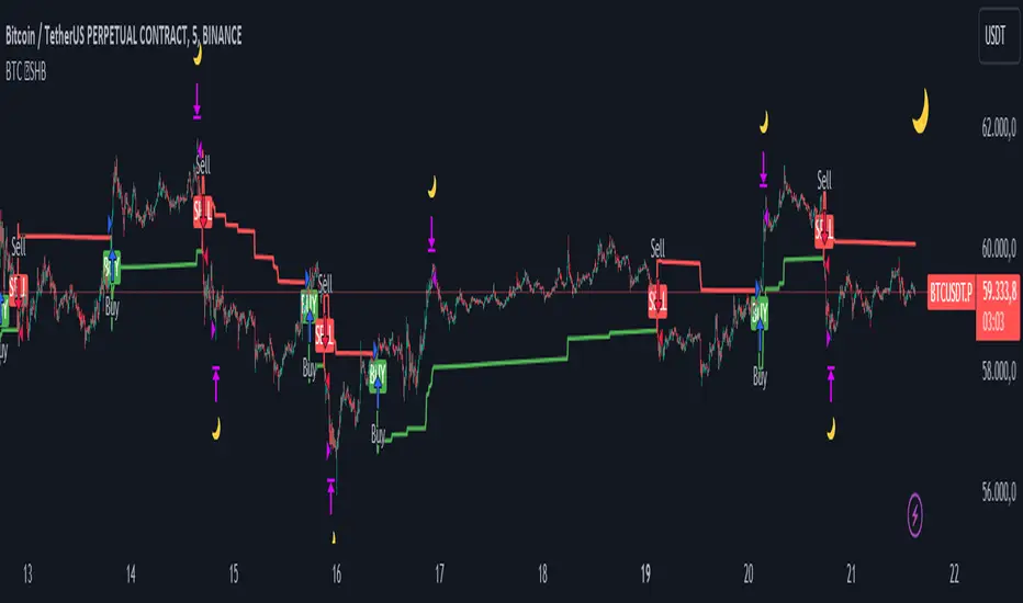
Gann + Laplace Smoothed Hybrid Volume Spread AnalysisThe Gann + Laplace Smoothed Hybrid Volume Spread Analysis ( GannLSHVSA ) Strategy/Indicator is an trading tool designed to fuse volume analysis with trend detection, offering traders a view of market dynamics.
This Strategy/Indicator stands apart by integrating the principles of the upgraded Discrete Fourier Transform (DFT), the Laplace Stieltjes Transform and volume spread analysis, enhanced with a layer of Fourier smoothing to distill market noise and highlight trend directions with unprecedented clarity.
The length of EMA and Strategy Entries are modified with the Gann swings .
This smoothing process allows traders to discern the true underlying patterns in volume and price action, stripped of the distractions of short-term fluctuations and noise.
The core functionality of the GannLSHVSA revolves around the innovative combination of volume change analysis, spread determination (calculated from the open and close price difference), and the strategic use of the EMA (default 10) to fine-tune the analysis of spread by incorporating volume changes.
Trend direction is validated through a moving average (MA) of the histogram, which acts analogously to the Volume MA found in traditional volume indicators. This MA serves as a pivotal reference point, enabling traders to confidently engage with the market when the histogram's movement concurs with the trend direction, particularly when it crosses the Trend MA line, signalling optimal entry points.
It returns 0 when MA of the histogram and EMA of the Price Spread are not align.
WHAT IS GannLSHVSA INDICATOR:
The GannLSHVSA plots a positive trend when a positive Volume smoothed Spread and EMA of Volume smoothed price is above 0, and a negative when negative Volume smoothed Spread and EMA of Volume smoothed price is below 0. When this conditions are not met it plots 0.
HOW TO USE THE STRATEGY:
Here you fine-tune the inputs until you find a combination that works well on all Timeframes you will use when creating your Automated Trade Algorithmic Strategy. I suggest 4h, 12h, 1D, 2D, 3D, 4D, 5D, 6D, W and M.
ORIGINALITY & USEFULNESS:
The GannLSHVSA Strategy is unique because it applies upgraded DFT, the Laplace Stieltjes Transform for data smoothing, effectively filtering out the minor fluctuations and leaving traders with a clear picture of the market's true movements. The DFT's ability to break down market signals into constituent frequencies offers a granular view of market dynamics, highlighting the amplitude and phase of each frequency component. This, combined with the strategic application of Ehler's Universal Oscillator principles via a histogram, furnishes traders with a nuanced understanding of market volatility and noise levels, thereby facilitating more informed trading decisions. The Gann swing strategy is developed by meomeo105, this Gann high and low algorithm forms the basis of the EMA modification.
DETAILED DESCRIPTION:
My detailed description of the indicator and use cases which I find very valuable.
What is the meaning of price spread?
In finance, a spread refers to the difference between two prices, rates, or yields. One of the most common types is the bid-ask spread, which refers to the gap between the bid (from buyers) and the ask (from sellers) prices of a security or asset.
We are going to use Open-Close spread.
What is Volume spread analysis?
Volume spread analysis (VSA) is a method of technical analysis that compares the volume per candle, range spread, and closing price to determine price direction.
What does this mean?
We need to have a positive Volume Price Spread and a positive Moving average of Volume price spread for a positive trend. OR via versa a negative Volume Price Spread and a negative Moving average of Volume price spread for a negative trend.
What if we have a positive Volume Price Spread and a negative Moving average of Volume Price Spread?
It results in a neutral, not trending price action.
Thus the Indicator/Strategy returns 0 and Closes all long and short positions.
I suggest using "Close all" input False when fine-tuning Inputs for 1 TimeFrame. When you export data to Excel/Numbers/GSheets I suggest using "Close all" input as True, except for the lowest TimeFrame. I suggest using 100% equity as your default quantity for fine-tune purposes. I have to mention that 100% equity may lead to unrealistic backtesting results. Be avare. When backtesting for trading purposes use Contracts or USDT.
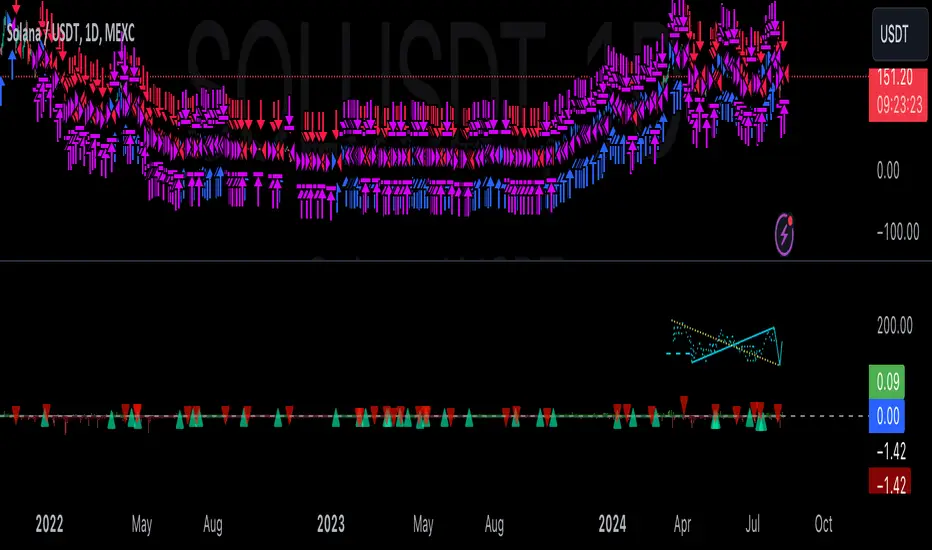
Dual Chain StrategyDual Chain Strategy - Technical Overview
How It Works:
The Dual Chain Strategy is a unique approach to trading that utilizes Exponential Moving Averages (EMAs) across different timeframes, creating two distinct "chains" of trading signals. These chains can work independently or together, capturing both long-term trends and short-term price movements.
Chain 1 (Longer-Term Focus):
Entry Signal: The entry signal for Chain 1 is generated when the closing price crosses above the EMA calculated on a weekly timeframe. This suggests the start of a bullish trend and prompts a long position.
bullishChain1 = enableChain1 and ta.crossover(src1, entryEMA1)
Exit Signal: The exit signal is triggered when the closing price crosses below the EMA on a daily timeframe, indicating a potential bearish reversal.
exitLongChain1 = enableChain1 and ta.crossunder(src1, exitEMA1)
Parameters: Chain 1's EMA length is set to 10 periods by default, with the flexibility for user adjustment to match various trading scenarios.
Chain 2 (Shorter-Term Focus):
Entry Signal: Chain 2 generates an entry signal when the closing price crosses above the EMA on a 12-hour timeframe. This setup is designed to capture quicker, shorter-term movements.
bullishChain2 = enableChain2 and ta.crossover(src2, entryEMA2)
Exit Signal: The exit signal occurs when the closing price falls below the EMA on a 9-hour timeframe, indicating the end of the shorter-term trend.
exitLongChain2 = enableChain2 and ta.crossunder(src2, exitEMA2)
Parameters: Chain 2's EMA length is set to 9 periods by default, and can be customized to better align with specific market conditions or trading strategies.
Key Features:
Dual EMA Chains: The strategy's originality shines through its dual-chain configuration, allowing traders to monitor and react to both long-term and short-term market trends. This approach is particularly powerful as it combines the strengths of trend-following with the agility of momentum trading.
Timeframe Flexibility: Users can modify the timeframes for both chains, ensuring the strategy can be tailored to different market conditions and individual trading styles. This flexibility makes it versatile for various assets and trading environments.
Independent Trade Logic: Each chain operates independently, with its own set of entry and exit rules. This allows for simultaneous or separate execution of trades based on the signals from either or both chains, providing a robust trading system that can handle different market phases.
Backtesting Period: The strategy includes a configurable backtesting period, enabling thorough performance assessment over a historical range. This feature is crucial for understanding how the strategy would have performed under different market conditions.
time_cond = time >= startDate and time <= finishDate
What It Does:
The Dual Chain Strategy offers traders a distinctive trading tool that merges two separate EMA-based systems into one cohesive framework. By integrating both long-term and short-term perspectives, the strategy enhances the ability to adapt to changing market conditions. The originality of this script lies in its innovative dual-chain design, providing traders with a unique edge by allowing them to capitalize on both significant trends and smaller, faster price movements.
Whether you aim to capture extended market trends or take advantage of more immediate price action, the Dual Chain Strategy provides a comprehensive solution with a high degree of customization and strategic depth. Its flexibility and originality make it a valuable tool for traders seeking to refine their approach to market analysis and execution.
How to Use the Dual Chain Strategy
Step 1: Access the Strategy
Add the Script: Start by adding the Dual Chain Strategy to your TradingView chart. You can do this by searching for the script by name or using the link provided.
Select the Asset: Apply the strategy to your preferred trading pair or asset, such as #BTCUSD, to see how it performs.
Step 2: Configure the Settings
Enable/Disable Chains:
The strategy is designed with two independent chains. You can choose to enable or disable each chain depending on your trading style and the market conditions.
enableChain1 = input.bool(true, title='Enable Chain 1')
enableChain2 = input.bool(true, title='Enable Chain 2')
By default, both chains are enabled. If you prefer to focus only on longer-term trends, you might disable Chain 2, or vice versa if you prefer shorter-term trades.
Set EMA Lengths:
Adjust the EMA lengths for each chain to match your trading preferences.
Chain 1: The default EMA length is 10 periods. This chain uses a weekly timeframe for entry signals and a daily timeframe for exits.
len1 = input.int(10, minval=1, title='Length Chain 1 EMA', group="Chain 1")
Chain 2: The default EMA length is 9 periods. This chain uses a 12-hour timeframe for entries and a 9-hour timeframe for exits.
len2 = input.int(9, minval=1, title='Length Chain 2 EMA', group="Chain 2")
Customize Timeframes:
You can customize the timeframes used for entry and exit signals for both chains.
Chain 1:
Entry Timeframe: Weekly
Exit Timeframe: Daily
tf1_entry = input.timeframe("W", title='Chain 1 Entry Timeframe', group="Chain 1")
tf1_exit = input.timeframe("D", title='Chain 1 Exit Timeframe', group="Chain 1")
Chain 2:
Entry Timeframe: 12 Hours
Exit Timeframe: 9 Hours
tf2_entry = input.timeframe("720", title='Chain 2 Entry Timeframe (12H)', group="Chain 2")
tf2_exit = input.timeframe("540", title='Chain 2 Exit Timeframe (9H)', group="Chain 2")
Set the Backtesting Period:
Define the period over which you want to backtest the strategy. This allows you to see how the strategy would have performed historically.
startDate = input.time(timestamp('2015-07-27'), title="StartDate")
finishDate = input.time(timestamp('2026-01-01'), title="FinishDate")
Step 3: Analyze the Signals
Understand the Entry and Exit Signals:
Buy Signals: When the price crosses above the entry EMA, the strategy generates a buy signal.
bullishChain1 = enableChain1 and ta.crossover(src1, entryEMA1)
Sell Signals: When the price crosses below the exit EMA, the strategy generates a sell signal.
bearishChain2 = enableChain2 and ta.crossunder(src2, entryEMA2)
Review the Visual Indicators:
The strategy plots buy and sell signals on the chart with labels for easy identification:
BUY C1/C2 for buy signals from Chain 1 and Chain 2.
SELL C1/C2 for sell signals from Chain 1 and Chain 2.
This visual aid helps you quickly understand when and why trades are being executed.
Step 4: Optimize the Strategy
Backtest Results:
Review the strategy’s performance over the backtesting period. Look at key metrics like net profit, drawdown, and trade statistics to evaluate its effectiveness.
Adjust the EMA lengths, timeframes, and other settings to see how changes affect the strategy’s performance.
Customize for Live Trading:
Once satisfied with the backtest results, you can apply the strategy settings to live trading. Remember to continuously monitor and adjust as needed based on market conditions.
Step 5: Implement Risk Management
Use Realistic Position Sizing:
Keep your risk exposure per trade within a comfortable range, typically between 1-2% of your trading capital.
Set Alerts:
Set up alerts for buy and sell signals, so you don’t miss trading opportunities.
Paper Trade First:
Consider running the strategy in a paper trading account to understand its behavior in real market conditions before committing real capital.
This dual-layered approach offers a distinct advantage: it enables the strategy to adapt to varying market conditions by capturing both broad trends and immediate price action without one chain's activity impacting the other's decision-making process. The independence of these chains in executing transactions adds a level of sophistication and flexibility that is rarely seen in more conventional trading systems, making the Dual Chain Strategy not just unique, but a powerful tool for traders seeking to navigate complex market environments.
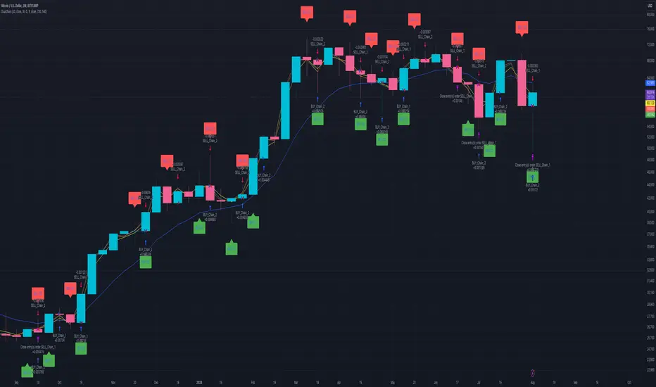
Fractal Breakout Trend Following StrategyOverview
The Fractal Breakout Trend Following Strategy is a trend-following system which utilizes the Willams Fractals and Alligator to execute the long trades on the fractal's breakouts which have a high probability to be the new uptrend phase beginning. This system also uses the normalized Average True Range indicator to filter trades after a large moves, because it's more likely to see the trend continuation after a consolidation period. Strategy can execute only long trades.
Unique Features
Trend and volatility filtering system: Strategy uses Williams Alligator to filter the counter-trend fractals breakouts and normalized Average True Range to avoid the trades after large moves, when volatility is high
Configurable Trading Periods: Users can tailor the strategy to specific market windows, adapting to different market conditions.
Flexible Risk Management: Users can choose the stop-loss percent (by default = 3%) for trades, but strategy also has the dynamic stop-loss level using down fractals.
Methodology
The strategy places stop order at the last valid fractal breakout level. Validity of this fractal is defined by the Williams Alligator indicator. If at the moment of time when price breaking the last fractal price is higher than Alligator's teeth line (8 period SMA shifted 5 bars in the future) this is a valid breakout. Moreover strategy has the additional volatility filtering system using normalized ATR. It calculates the average normalized ATR for last user-defined number of bars and if this value lower than the user-defined threshold value the long trade is executed.
When trade is opened, script places the stop loss at the price higher of two levels: user defined stop-loss from the position entry price or down fractal validation level. The down fractal is valid with the rule, opposite as the up fractal validation. Price shall break to the downside the last down fractal below the Willians Alligator's teeth line.
Strategy has no fixed take profit. Exit level changes with the down fractal validation level. If price is in strong uptrend trade is going to be active until last down fractal is not valid. Strategy closes trade when price hits the down fractal validation level.
Risk Management
The strategy employs a combined approach to risk management:
It allows positions to ride the trend as long as the price continues to move favorably, aiming to capture significant price movements. It features a user-defined stop-loss parameter to mitigate risks based on individual risk tolerance. By default, this stop-loss is set to a 3% drop from the entry point, but it can be adjusted according to the trader's preferences.
Justification of Methodology
This strategy leverages Williams Fractals to open long trade when price has broken the key resistance level to the upside. This resistance level is the last up fractal and is shall be broken above the Williams Alligator's teeth line to be qualified as the valid breakout according to this strategy. The Alligator filtering increases the probability to avoid the false breakouts against the current trend.
Moreover strategy has an additional filter using Average True Range(ATR) indicator. If average value of ATR for the last user-defined number of bars is lower than user-defined threshold strategy can open the long trade according to open trade condition above. The logic here is following: we want to open trades after period of price consolidation inside the range because before and after a big move price is more likely to be in sideways, but we need a trend move to have a profit.
Another one important feature is how the exit condition is defined. On the one hand, strategy has the user-defined stop-loss (3% below the entry price by default). It's made to give users the opportunity to restrict their losses according to their risk-tolerance. On the other hand, strategy utilizes the dynamic exit level which is defined by down fractal activation. If we assume the breaking up fractal is the beginning of the uptrend, breaking down fractal can be the start of downtrend phase. We don't want to be in long trade if there is a high probability of reversal to the downside. This approach helps to not keep open trade if trend is not developing and hold it if price continues going up.
Backtest Results
Operating window: Date range of backtests is 2023.01.01 - 2024.05.01. It is chosen to let the strategy to close all opened positions.
Commission and Slippage: Includes a standard Binance commission of 0.1% and accounts for possible slippage over 5 ticks.
Initial capital: 10000 USDT
Percent of capital used in every trade: 30%
Maximum Single Position Loss: -3.19%
Maximum Single Profit: +24.97%
Net Profit: +3036.90 USDT (+30.37%)
Total Trades: 83 (28.92% win rate)
Profit Factor: 1.953
Maximum Accumulated Loss: 963.98 USDT (-8.29%)
Average Profit per Trade: 36.59 USDT (+1.12%)
Average Trade Duration: 72 hours
These results are obtained with realistic parameters representing trading conditions observed at major exchanges such as Binance and with realistic trading portfolio usage parameters.
How to Use
Add the script to favorites for easy access.
Apply to the desired timeframe and chart (optimal performance observed on 4h and higher time frames and the BTC/USDT).
Configure settings using the dropdown choice list in the built-in menu.
Set up alerts to automate strategy positions through web hook with the text: {{strategy.order.alert_message}}
Disclaimer:
Educational and informational tool reflecting Skyrex commitment to informed trading. Past performance does not guarantee future results. Test strategies in a simulated environment before live implementation

Fine-Tune Inputs: Fourier Smoothed Hybrid Volume Spread AnalysisUse this Strategy to Fine-tune inputs for the HSHVSA Indicator.
Strategy allows you to fine-tune the indicator for 1 TimeFrame at a time; cross Timeframe Input fine-tuning is done manually after exporting the chart data.
I suggest using " Close all " input False when fine-tuning Inputs for 1 TimeFrame. When you export data to Excel/Numbers/GSheets I suggest using " Close all " input as True , except for the lowest TimeFrame.
MEANINGFUL DESCRIPTION:
The Fourier Smoothed Hybrid Volume Spread Analysis (FSHVSA) Strategy/Indicator is an innovative trading tool designed to fuse volume analysis with trend detection capabilities, offering traders a comprehensive view of market dynamics.
This Strategy/Indicator stands apart by integrating the principles of the Discrete Fourier Transform (DFT) and volume spread analysis, enhanced with a layer of Fourier smoothing to distill market noise and highlight trend directions with unprecedented clarity.
This smoothing process allows traders to discern the true underlying patterns in volume and price action, stripped of the distractions of short-term fluctuations and noise.
The core functionality of the FSHVSA revolves around the innovative combination of volume change analysis, spread determination (calculated from the open and close price difference), and the strategic use of the EMA (default 10) to fine-tune the analysis of spread by incorporating volume changes.
Trend direction is validated through a moving average (MA) of the histogram, which acts analogously to the Volume MA found in traditional volume indicators. This MA serves as a pivotal reference point, enabling traders to confidently engage with the market when the histogram's movement concurs with the trend direction, particularly when it crosses the Trend MA line, signalling optimal entry points.
It returns 0 when MA of the histogram and EMA of the Price Spread are not align.
WHAT IS FSHVSA INDICATOR:
The FSHVSA plots a positive trend when a positive Volume smoothed Spread and EMA of Volume smoothed price is above 0, and a negative when negative Volume smoothed Spread and EMA of Volume smoothed price is below 0. When this conditions are not met it plots 0.
HOW TO USE THE STRATEGY:
Here you fine-tune the inputs until you find a combination that works well on all Timeframes you will use when creating your Automated Trade Algorithmic Strategy. I suggest 4h, 12h, 1D, 2D, 3D, 4D, 5D, 6D, W and M.
ORIGINALITY & USEFULNESS:
The FSHVSA Strategy is unique because it applies DFT for data smoothing, effectively filtering out the minor fluctuations and leaving traders with a clear picture of the market's true movements. The DFT's ability to break down market signals into constituent frequencies offers a granular view of market dynamics, highlighting the amplitude and phase of each frequency component. This, combined with the strategic application of Ehler's Universal Oscillator principles via a histogram, furnishes traders with a nuanced understanding of market volatility and noise levels, thereby facilitating more informed trading decisions.
DETAILED DESCRIPTION:
My detailed description of the indicator and use cases which I find very valuable.
What is the meaning of price spread?
In finance, a spread refers to the difference between two prices, rates, or yields. One of the most common types is the bid-ask spread, which refers to the gap between the bid (from buyers) and the ask (from sellers) prices of a security or asset.
We are going to use Open-Close spread.
What is Volume spread analysis?
Volume spread analysis (VSA) is a method of technical analysis that compares the volume per candle, range spread, and closing price to determine price direction.
What does this mean?
We need to have a positive Volume Price Spread and a positive Moving average of Volume price spread for a positive trend. OR via versa a negative Volume Price Spread and a negative Moving average of Volume price spread for a negative trend.
What if we have a positive Volume Price Spread and a negative Moving average of Volume Price Spread?
It results in a neutral, not trending price action.
Thus the Indicator/Strategy returns 0 and Closes all long and short positions.
In the next Image you can see that trend is negative on 4h, we just move Negative on 12h and Positive on 1D. That means trend/Strategy flipped negative .
I am sorry, the chart is a bit messy. The idea is to use the indicator/strategy over more than 1 Timeframe.
Use this Strategy to fine-tune inputs for the HSHVSA Indicator.
(Strategy allows you to fine-tune the indicator for 1 TimeFrame at a time; cross Timeframe Input fine-tuning is done manually after exporting the chart data)
I suggest using " Close all " input False when fine-tuning Inputs for 1 TimeFrame. When you export data to Excel/Numbers/GSheets I suggest using " Close all " input as True , except for the lowest TimeFrame. I suggest using 100% equity as your default quantity for fine-tune purposes. I have to mention that 100% equity may lead to unrealistic backtesting results. Be avare. When backtesting for trading purposes use Contracts or USDT.

TrippleMACDCryptocurrency Scalping Strategy for 1m Timeframe
Introduction:
Welcome to our cutting-edge cryptocurrency scalping strategy tailored specifically for the 1-minute timeframe. By combining three MACD indicators with different parameters and averaging them, along with applying RSI, we've developed a highly effective strategy for maximizing profits in the cryptocurrency market. This strategy is designed for automated trading through our bot, which executes trades using hooks. All trades are calculated for long positions only, ensuring optimal performance in a fast-paced market.
Key Components:
MACD (Moving Average Convergence Divergence):
We've utilized three MACD indicators with varying parameters to capture different aspects of market momentum.
Averaging these MACD indicators helps smooth out noise and provides a more reliable signal for trading decisions.
RSI (Relative Strength Index):
RSI serves as a complementary indicator, providing insights into the strength of bullish trends.
By incorporating RSI, we enhance the accuracy of our entry and exit points, ensuring timely execution of trades.
Strategy Overview:
Long Position Entries:
Initiate long positions when all three MACD indicators signal bullish momentum and the RSI confirms bullish strength.
This combination of indicators increases the probability of successful trades, allowing us to capitalize on uptrends effectively.
Utilizing Linear Regression:
Linear regression is employed to identify consolidation phases in the market.
Recognizing consolidation periods helps us avoid trading during choppy price action, ensuring optimal performance.
Suitability for Grid Trading Bots:
Our strategy is well-suited for grid trading bots due to frequent price fluctuations and opportunities for grid activation.
The strategy's design accounts for price breakthroughs, which are advantageous for grid trading strategies.
Benefits of the Strategy:
Consistent Performance Across Cryptocurrencies:
Through rigorous testing on various cryptocurrency futures contracts, our strategy has demonstrated favorable results across different coins.
Its adaptability makes it a versatile tool for traders seeking consistent profits in the cryptocurrency market.
Integration of Advanced Techniques:
By integrating multiple indicators and employing linear regression, our strategy leverages advanced techniques to enhance trading performance.
This strategic approach ensures a comprehensive analysis of market conditions, leading to well-informed trading decisions.
Conclusion:
Our cryptocurrency scalping strategy offers a sophisticated yet user-friendly approach to trading in the fast-paced environment of the 1-minute timeframe. With its emphasis on automation, accuracy, and adaptability, our strategy empowers traders to navigate the complexities of the cryptocurrency market with confidence. Whether you're a seasoned trader or a novice investor, our strategy provides a reliable framework for achieving consistent profits and maximizing returns on your investment.

Bitcoin 5A Strategy@LilibtcIn our long-term strategy, we have deeply explored the key factors influencing the price of Bitcoin. By precisely calculating the correlation between these factors and the price of Bitcoin, we found that they are closely linked to the value of Bitcoin. To more effectively predict the fair price of Bitcoin, we have built a predictive model and adjusted our investment strategy accordingly based on this model. In practice, the prediction results of this model correspond quite high with actual values, fully demonstrating its reliability in predicting price fluctuations.
When the future is uncertain and the outlook is unclear, people often choose to hold back and avoid risks, or even abandon their original plans. However, the prediction of Bitcoin is full of challenges, but we have taken the first step in exploring.
Table of contents:
Usage Guide
Step 1: Identify the factors that have the greatest impact on Bitcoin price
Step 2: Build a Bitcoin price prediction model
Step 3: Find indicators for warning of bear market bottoms and bull market tops
Step 4: Predict Bitcoin Price in 2025
Step 5: Develop a Bitcoin 5A strategy
Step 6: Verify the performance of the Bitcoin 5A strategy
Usage Restrictions
🦮Usage Guide:
1. On the main interface, modify the code, find the BTCUSD trading pair, and select the BITSTAMP exchange for trading.
2. Set the time period to the daily chart.
3. Select a logarithmic chart in the chart type to better identify price trends.
4. In the strategy settings, adjust the options according to personal needs, including language, display indicators, display strategies, display performance, display optimizations, sell alerts, buy prompts, opening days, backtesting start year, backtesting start month, and backtesting start date.
🏃Step 1: Identify the factors that have the greatest impact on Bitcoin price
📖Correlation Coefficient: A mathematical concept for measuring influence
In order to predict the price trend of Bitcoin, we need to delve into the factors that have the greatest impact on its price. These factors or variables can be expressed in mathematical or statistical correlation coefficients. The correlation coefficient is an indicator of the degree of association between two variables, ranging from -1 to 1. A value of 1 indicates a perfect positive correlation, while a value of -1 indicates a perfect negative correlation.
For example, if the price of corn rises, the price of live pigs usually rises accordingly, because corn is the main feed source for pig breeding. In this case, the correlation coefficient between corn and live pig prices is approximately 0.3. This means that corn is a factor affecting the price of live pigs. On the other hand, if a shooter's performance improves while another shooter's performance deteriorates due to increased psychological pressure, we can say that the former is a factor affecting the latter's performance.
Therefore, in order to identify the factors that have the greatest impact on the price of Bitcoin, we need to find the factors with the highest correlation coefficients with the price of Bitcoin. If, through the analysis of the correlation between the price of Bitcoin and the data on the chain, we find that a certain data factor on the chain has the highest correlation coefficient with the price of Bitcoin, then this data factor on the chain can be identified as the factor that has the greatest impact on the price of Bitcoin. Through calculation, we found that the 🔵number of Bitcoin blocks is one of the factors that has the greatest impact on the price of Bitcoin. From historical data, it can be clearly seen that the growth rate of the 🔵number of Bitcoin blocks is basically consistent with the movement direction of the price of Bitcoin. By analyzing the past ten years of data, we obtained a daily correlation coefficient of 0.93 between the number of Bitcoin blocks and the price of Bitcoin.
🏃Step 2: Build a Bitcoin price prediction model
📖Predictive Model: What formula is used to predict the price of Bitcoin?
Among various prediction models, the linear function is the preferred model due to its high accuracy. Take the standard weight as an example, its linear function graph is a straight line, which is why we choose the linear function model. However, the growth rate of the price of Bitcoin and the number of blocks is extremely fast, which does not conform to the characteristics of the linear function. Therefore, in order to make them more in line with the characteristics of the linear function, we first take the logarithm of both. By observing the logarithmic graph of the price of Bitcoin and the number of blocks, we can find that after the logarithm transformation, the two are more in line with the characteristics of the linear function. Based on this feature, we choose the linear regression model to establish the prediction model.
From the graph below, we can see that the actual red and green K-line fluctuates around the predicted blue and 🟢green line. These predicted values are based on fundamental factors of Bitcoin, which support its value and reflect its reasonable value. This picture is consistent with the theory proposed by Marx in "Das Kapital" that "prices fluctuate around values."
The predicted logarithm of the market cap of Bitcoin is calculated through the model. The specific calculation formula of the Bitcoin price prediction value is as follows:
btc_predicted_marketcap = math.exp(btc_predicted_marketcap_log)
btc_predicted_price = btc_predicted_marketcap / btc_supply
🏃Step 3: Find indicators for early warning of bear market bottoms and bull market tops
📖Warning Indicator: How to Determine Whether the Bitcoin Price has Reached the Bear Market Bottom or the Bull Market Top?
By observing the Bitcoin price logarithmic prediction chart mentioned above, we notice that the actual price often falls below the predicted value at the bottom of a bear market; during the peak of a bull market, the actual price exceeds the predicted price. This pattern indicates that the deviation between the actual price and the predicted price can serve as an early warning signal. When the 🔴 Bitcoin price deviation is very low, as shown by the chart with 🟩green background, it usually means that we are at the bottom of the bear market; Conversely, when the 🔴 Bitcoin price deviation is very high, the chart with a 🟥red background indicates that we are at the peak of the bull market.
This pattern has been validated through six bull and bear markets, and the deviation value indeed serves as an early warning signal, which can be used as an important reference for us to judge market trends.
🏃Step 4:Predict Bitcoin Price in 2025
📖Price Upper Limit
According to the data calculated on February 25, 2024, the 🟠upper limit of the Bitcoin price is $194,287, which is the price ceiling of this bull market. The peak of the last bull market was on November 9, 2021, at $68,664. The bull-bear market cycle is 4 years, so the highest point of this bull market is expected in 2025. That is where you should sell the Bitcoin. and the upper limit of the Bitcoin price will exceed $190,000. The closing price of Bitcoin on February 25, 2024, was $51,729, with an expected increase of 2.7 times.
🏃Step 5: Bitcoin 5A Strategy Formulation
📖Strategy: When to buy or sell, and how many to choose?
We introduce the Bitcoin 5A strategy. This strategy requires us to generate trading signals based on the critical values of the warning indicators, simulate the trades, and collect performance data for evaluation. In the Bitcoin 5A strategy, there are three key parameters: buying warning indicator, batch trading days, and selling warning indicator. Batch trading days are set to ensure that we can make purchases in batches after the trading signal is sent, thus buying at a lower price, selling at a higher price, and reducing the trading impact cost.
In order to find the optimal warning indicator critical value and batch trading days, we need to adjust these parameters repeatedly and perform backtesting. Backtesting is a method established by observing historical data, which can help us better understand market trends and trading opportunities.
Specifically, we can find the key trading points by watching the Bitcoin price log and the Bitcoin price deviation chart. For example, on August 25, 2015, the 🔴 Bitcoin price deviation was at its lowest value of -1.11; on December 17, 2017, the 🔴 Bitcoin price deviation was at its highest value at the time, 1.69; on March 16, 2020, the 🔴 Bitcoin price deviation was at its lowest value at the time, -0.91; on March 13, 2021, the 🔴 Bitcoin price deviation was at its highest value at the time, 1.1; on December 31, 2022, the 🔴 Bitcoin price deviation was at its lowest value at the time, -1.
To ensure that all five key trading points generate trading signals, we set the warning indicator Bitcoin price deviation to the larger of the three lowest values, -0.9, and the smallest of the two highest values, 1. Then, we buy when the warning indicator Bitcoin price deviation is below -0.9, and sell when it is above 1.
In addition, we set the batch trading days as 25 days to implement a strategy that averages purchases and sales. Within these 25 days, we will invest all funds into the market evenly, buying once a day. At the same time, we also sell positions at the same pace, selling once a day.
📖Adjusting the threshold: a key step to optimizing trading strategy
Adjusting the threshold is an indispensable step for better performance. Here are some suggestions for adjusting the batch trading days and critical values of warning indicators:
• Batch trading days: Try different days like 25 to see how it affects overall performance.
• Buy and sell critical values for warning indicators: iteratively fine-tune the buy threshold value of -0.9 and the sell threshold value of 1 exhaustively to find the best combination of threshold values.
Through such careful adjustments, we may find an optimized approach with a lower maximum drawdown rate (e.g., 11%) and a higher cumulative return rate for closed trades (e.g., 474 times). The chart below is a backtest optimization chart for the Bitcoin 5A strategy, providing an intuitive display of strategy adjustments and optimizations.
In this way, we can better grasp market trends and trading opportunities, thereby achieving a more robust and efficient trading strategy.
🏃Step 6: Validating the performance of the Bitcoin 5A Strategy
📖Model interpretability validation: How to explain the Bitcoin price model?
The interpretability of the model is represented by the coefficient of determination R squared, which reflects the degree of match between the predicted value and the actual value. I divided all the historical data from August 18, 2015 into two groups, and used the data from August 18, 2011 to August 18, 2015 as training data to generate the model. The calculation result shows that the coefficient of determination R squared during the 2011-2015 training period is as high as 0.81, which shows that the interpretability of this model is quite high. From the Bitcoin price logarithmic prediction chart in the figure below, we can see that the deviation between the predicted value and the actual value is not far, which means that most of the predicted values can explain the actual value well.
The calculation formula for the coefficient of determination R squared is as follows:
residual = btc_close_log - btc_predicted_price_log
residual_square = residual * residual
train_residual_square_sum = math.sum(residual_square, train_days)
train_mse = train_residual_square_sum / train_days
train_r2 = 1 - train_mse / ta.variance(btc_close_log, train_days)
📖Model stability verification: How to affirm the stability of the Bitcoin price model when new data is available?
Model stability is achieved through model verification. I set the last day of the training period to February 2, 2024 as the "verification group" and used it as verification data to verify the stability of the model. This means that after generating the model if there is new data, I will use these new data together with the model for prediction, and then evaluate the interpretability of the model. If the coefficient of determination when using verification data is close to the previous training one and both remain at a high level, then we can consider this model as stability. The coefficient of determination calculated from the validation period data and model prediction results is as high as 0.83, which is close to the previous 0.81, further proving the stability of this model.
📖Performance evaluation: How to accurately evaluate historical backtesting results?
After detailed strategy testing, to ensure the accuracy and reliability of the results, we need to carry out a detailed performance evaluation on the backtest results. The key evaluation indices include:
• Net value curve: As shown in the rose line, it intuitively reflects the growth of the account net value. By observing the net value curve, we can understand the overall performance and profitability of the strategy.
The basic attributes of this strategy are as follows:
Trading range: 2015-8-19 to 2024-2-18, backtest range: 2011-8-18 to 2024-2-18
Initial capital: 1000USD, order size: 1 contract, pyramid: 50 orders, commission rate: 0.2%, slippage: 20 markers.
In the strategy tester overview chart, we also obtained the following key data:
• Net profit rate of closed trades: as high as 474 times, far exceeding the benchmark, as shown in the strategy tester performance summary chart, Bitcoin buys and holds 210 times.
• Number of closed trades and winning percentage: 100 trades were all profitable, showing the stability and reliability of the strategy.
• Drawdown rate & win-loose ratio: The maximum drawdown rate is only 11%, far lower than Bitcoin's 78%. Profit factor, or win-loose ratio, reached 500, further proving the advantage of the strategy.
Through these detailed evaluations, we can see clearly the excellent balance between risk and return of the Bitcoin 5A strategy.
⚠️Usage Restrictions: Strategy Application in Specific Situations
Please note that this strategy is designed specifically for Bitcoin and should not be applied to other assets or markets without authorization. In actual operations, we should make careful decisions according to our risk tolerance and investment goals.

Bitcoin 5A Strategy - Price Upper & Lower Limit@LilibtcIn our long-term strategy, we have deeply explored the key factors influencing the price of Bitcoin. By precisely calculating the correlation between these factors and the price of Bitcoin, we found that they are closely linked to the value of Bitcoin. To more effectively predict the fair price of Bitcoin, we have built a predictive model and adjusted our investment strategy accordingly based on this model. In practice, the prediction results of this model correspond quite high with actual values, fully demonstrating its reliability in predicting price fluctuations.
When the future is uncertain and the outlook is unclear, people often choose to hold back and avoid risks, or even abandon their original plans. However, the prediction of Bitcoin is full of challenges, but we have taken the first step in exploring.
Table of contents:
Usage Guide
Step 1: Identify the factors that have the greatest impact on Bitcoin price
Step 2: Build a Bitcoin price prediction model
Step 3: Find indicators for warning of bear market bottoms and bull market tops
Step 4: Predict Bitcoin Price in 2025
Step 5: Develop a Bitcoin 5A strategy
Step 6: Verify the performance of the Bitcoin 5A strategy
Usage Restrictions
🦮Usage Guide:
1. On the main interface, modify the code, find the BTCUSD trading pair, and select the BITSTAMP exchange for trading.
2. Set the time period to the daily chart.
3. Select a logarithmic chart in the chart type to better identify price trends.
4. In the strategy settings, adjust the options according to personal needs, including language, display indicators, display strategies, display performance, display optimizations, sell alerts, buy prompts, opening days, backtesting start year, backtesting start month, and backtesting start date.
🏃Step 1: Identify the factors that have the greatest impact on Bitcoin price
📖Correlation Coefficient: A mathematical concept for measuring influence
In order to predict the price trend of Bitcoin, we need to delve into the factors that have the greatest impact on its price. These factors or variables can be expressed in mathematical or statistical correlation coefficients. The correlation coefficient is an indicator of the degree of association between two variables, ranging from -1 to 1. A value of 1 indicates a perfect positive correlation, while a value of -1 indicates a perfect negative correlation.
For example, if the price of corn rises, the price of live pigs usually rises accordingly, because corn is the main feed source for pig breeding. In this case, the correlation coefficient between corn and live pig prices is approximately 0.3. This means that corn is a factor affecting the price of live pigs. On the other hand, if a shooter's performance improves while another shooter's performance deteriorates due to increased psychological pressure, we can say that the former is a factor affecting the latter's performance.
Therefore, in order to identify the factors that have the greatest impact on the price of Bitcoin, we need to find the factors with the highest correlation coefficients with the price of Bitcoin. If, through the analysis of the correlation between the price of Bitcoin and the data on the chain, we find that a certain data factor on the chain has the highest correlation coefficient with the price of Bitcoin, then this data factor on the chain can be identified as the factor that has the greatest impact on the price of Bitcoin. Through calculation, we found that the 🔵 number of Bitcoin blocks is one of the factors that has the greatest impact on the price of Bitcoin. From historical data, it can be clearly seen that the growth rate of the 🔵 number of Bitcoin blocks is basically consistent with the movement direction of the price of Bitcoin. By analyzing the past ten years of data, we obtained a daily correlation coefficient of 0.93 between the number of Bitcoin blocks and the price of Bitcoin.
🏃Step 2: Build a Bitcoin price prediction model
📖Predictive Model: What formula is used to predict the price of Bitcoin?
Among various prediction models, the linear function is the preferred model due to its high accuracy. Take the standard weight as an example, its linear function graph is a straight line, which is why we choose the linear function model. However, the growth rate of the price of Bitcoin and the number of blocks is extremely fast, which does not conform to the characteristics of the linear function. Therefore, in order to make them more in line with the characteristics of the linear function, we first take the logarithm of both. By observing the logarithmic graph of the price of Bitcoin and the number of blocks, we can find that after the logarithm transformation, the two are more in line with the characteristics of the linear function. Based on this feature, we choose the linear regression model to establish the prediction model.
From the graph below, we can see that the actual red and green K-line fluctuates around the predicted blue and 🟢green line. These predicted values are based on fundamental factors of Bitcoin, which support its value and reflect its reasonable value. This picture is consistent with the theory proposed by Marx in "Das Kapital" that "prices fluctuate around values."
The predicted logarithm of the market cap of Bitcoin is calculated through the model. The specific calculation formula of the Bitcoin price prediction value is as follows:
btc_predicted_marketcap = math.exp(btc_predicted_marketcap_log)
btc_predicted_price = btc_predicted_marketcap / btc_supply
🏃Step 3: Find indicators for early warning of bear market bottoms and bull market tops
📖Warning Indicator: How to Determine Whether the Bitcoin Price has Reached the Bear Market Bottom or the Bull Market Top?
By observing the Bitcoin price logarithmic prediction chart mentioned above, we notice that the actual price often falls below the predicted value at the bottom of a bear market; during the peak of a bull market, the actual price exceeds the predicted price. This pattern indicates that the deviation between the actual price and the predicted price can serve as an early warning signal. When the 🔴 Bitcoin price deviation is very low, as shown by the chart with 🟩green background, it usually means that we are at the bottom of the bear market; Conversely, when the 🔴 Bitcoin price deviation is very high, the chart with a 🟥red background indicates that we are at the peak of the bull market.
This pattern has been validated through six bull and bear markets, and the deviation value indeed serves as an early warning signal, which can be used as an important reference for us to judge market trends.
🏃Step 4:Predict Bitcoin Price in 2025
📖Price Upper Limit
According to the data calculated on March 10, 2023(If you want to check latest data, please contact with author), the 🟠upper limit of the Bitcoin price is $132,453, which is the price ceiling of this bull market. The peak of the last bull market was on November 9, 2021, at $68,664. The bull-bear market cycle is 4 years, so the highest point of this bull market is expected in 2025, and the 🟠upper limit of the Bitcoin price will exceed $130,000. The closing price of Bitcoin on March 10, 2024, was $68,515, with an expected increase of 90%.
🏃Step 5: Bitcoin 5A Strategy Formulation
📖Strategy: When to buy or sell, and how many to choose?
We introduce the Bitcoin 5A strategy. This strategy requires us to generate trading signals based on the critical values of the warning indicators, simulate the trades, and collect performance data for evaluation. In the Bitcoin 5A strategy, there are three key parameters: buying warning indicator, batch trading days, and selling warning indicator. Batch trading days are set to ensure that we can make purchases in batches after the trading signal is sent, thus buying at a lower price, selling at a higher price, and reducing the trading impact cost.
In order to find the optimal warning indicator critical value and batch trading days, we need to adjust these parameters repeatedly and perform backtesting. Backtesting is a method established by observing historical data, which can help us better understand market trends and trading opportunities.
Specifically, we can find the key trading points by watching the Bitcoin price log and the Bitcoin price deviation chart. For example, on August 25, 2015, the 🔴 Bitcoin price deviation was at its lowest value of -1.11; on December 17, 2017, the 🔴 Bitcoin price deviation was at its highest value at the time, 1.69; on March 16, 2020, the 🔴 Bitcoin price deviation was at its lowest value at the time, -0.91; on March 13, 2021, the 🔴 Bitcoin price deviation was at its highest value at the time, 1.1; on December 31, 2022, the 🔴 Bitcoin price deviation was at its lowest value at the time, -1.
To ensure that all five key trading points generate trading signals, we set the warning indicator Bitcoin price deviation to the larger of the three lowest values, -0.9, and the smallest of the two highest values, 1. Then, we buy when the warning indicator Bitcoin price deviation is below -0.9, and sell when it is above 1.
In addition, we set the batch trading days as 25 days to implement a strategy that averages purchases and sales. Within these 25 days, we will invest all funds into the market evenly, buying once a day. At the same time, we also sell positions at the same pace, selling once a day.
📖Adjusting the threshold: a key step to optimizing trading strategy
Adjusting the threshold is an indispensable step for better performance. Here are some suggestions for adjusting the batch trading days and critical values of warning indicators:
• Batch trading days: Try different days like 25 to see how it affects overall performance.
• Buy and sell critical values for warning indicators: iteratively fine-tune the buy threshold value of -0.9 and the sell threshold value of 1 exhaustively to find the best combination of threshold values.
Through such careful adjustments, we may find an optimized approach with a lower maximum drawdown rate (e.g., 11%) and a higher cumulative return rate for closed trades (e.g., 474 times). The chart below is a backtest optimization chart for the Bitcoin 5A strategy, providing an intuitive display of strategy adjustments and optimizations.
In this way, we can better grasp market trends and trading opportunities, thereby achieving a more robust and efficient trading strategy.
🏃Step 6: Validating the performance of the Bitcoin 5A Strategy
📖Model accuracy validation: How to judge the accuracy of the Bitcoin price model?
The accuracy of the model is represented by the coefficient of determination R square, which reflects the degree of match between the predicted value and the actual value. I divided all the historical data from August 18, 2015 into two groups, and used the data from August 18, 2011 to August 18, 2015 as training data to generate the model. The calculation result shows that the coefficient of determination R squared during the 2011-2015 training period is as high as 0.81, which shows that the accuracy of this model is quite high. From the Bitcoin price logarithmic prediction chart in the figure below, we can see that the deviation between the predicted value and the actual value is not far, which means that most of the predicted values can explain the actual value well.
The calculation formula for the coefficient of determination R square is as follows:
residual = btc_close_log - btc_predicted_price_log
residual_square = residual * residual
train_residual_square_sum = math.sum(residual_square, train_days)
train_mse = train_residual_square_sum / train_days
train_r2 = 1 - train_mse / ta.variance(btc_close_log, train_days)
📖Model reliability verification: How to affirm the reliability of the Bitcoin price model when new data is available?
Model reliability is achieved through model verification. I set the last day of the training period to February 2, 2024 as the "verification group" and used it as verification data to verify the reliability of the model. This means that after generating the model if there is new data, I will use these new data together with the model for prediction, and then evaluate the accuracy of the model. If the coefficient of determination when using verification data is close to the previous training one and both remain at a high level, then we can consider this model as reliable. The coefficient of determination calculated from the validation period data and model prediction results is as high as 0.83, which is close to the previous 0.81, further proving the reliability of this model.
📖Performance evaluation: How to accurately evaluate historical backtesting results?
After detailed strategy testing, to ensure the accuracy and reliability of the results, we need to carry out a detailed performance evaluation on the backtest results. The key evaluation indices include:
• Net value curve: As shown in the rose line, it intuitively reflects the growth of the account net value. By observing the net value curve, we can understand the overall performance and profitability of the strategy.
The basic attributes of this strategy are as follows:
Trading range: 2015-8-19 to 2024-2-18, backtest range: 2011-8-18 to 2024-2-18
Initial capital: 1000USD, order size: 1 contract, pyramid: 50 orders, commission rate: 0.2%, slippage: 20 markers.
In the strategy tester overview chart, we also obtained the following key data:
• Net profit rate of closed trades: as high as 474 times, far exceeding the benchmark, as shown in the strategy tester performance summary chart, Bitcoin buys and holds 210 times.
• Number of closed trades and winning percentage: 100 trades were all profitable, showing the stability and reliability of the strategy.
• Drawdown rate & win-loose ratio: The maximum drawdown rate is only 11%, far lower than Bitcoin's 78%. Profit factor, or win-loose ratio, reached 500, further proving the advantage of the strategy.
Through these detailed evaluations, we can see clearly the excellent balance between risk and return of the Bitcoin 5A strategy.
⚠️Usage Restrictions: Strategy Application in Specific Situations
Please note that this strategy is designed specifically for Bitcoin and should not be applied to other assets or markets without authorization. In actual operations, we should make careful decisions according to our risk tolerance and investment goals.

Strategy / Connectable [Azullian]The connectable strategy serves as a foundational component in our indicator system on TradingView, designed for intuitive testing, visualization, and construction of trading strategies. In concert with the connectable signal filter , it forms a cohesive unit that allows for efficient signal processing and strategy implementation. This integration enables the strategy to receive and act on weighted signals from various connectable indicators, making it a versatile tool for both novice and experienced traders.
Let's review the separate parts of this indicator.
█ STRATEGY INPUTS
We've provided an input to connect a signal filter or indicators or chains (→) which is set to 'Close' by default.
An input has several controls:
• Input: Connect indicators or signal filter here, choose indicators with a compatible : Signal connector.
• SM - Signal Mode: Choose a trading direction compatible with the settings in your signal filter
█ POSITION INVESTMENT
Determine the percentage of your trading budget you would like to use in each position based on the strategy's profit or loss.
• LINVB - Loss Investment Base: Choose which base to use to determine the investment percentage when the strategy is in a loss.
○ Equity: Use the equity as the base for percentage calculation.
○ Initial capital: Use the initial capital as the base for percentage calculation.
• LINV% - Loss Investment Percentage: Set a percentage of the chosen investment base as the investment for a new position.
○ For example, when 10% in loss, and a initial capital of $100, and the investment base is set to equity with a percentage of 50%, your investment will be 50% of $90, $45.
• PINVB - Profit Investment Base: Choose which base to use to determine the investment percentage when the strategy is in profit.
○ Equity: Use the equity as the base for percentage calculation.
○ Initial capital: Use the initial capital as the base for percentage calculation.
• PINV% - Profit Investment Percentage: Set a percentage of the chosen investment base as the investment for a new position.
○ For example, when 10% in profit, and an initial capital of $100, and the investment base is set to equity with a percentage of 100%, your investment will be 100% of $110, $110.
• RISK% - Risk Percentage:
○ Determine how much of the calculated position investment is at risk when the stop-loss is hit.
- For example, 1% of $45 represents a maximum loss of $0.45.
○ Risk percentage works together with the stop loss and the max leverage.
• MXLVG - Maximum Leverage:
○ Investigate the trading rules for your trading pair and use the maximum allowed amount of leverage.
○ To determine the number of contracts to be bought or sold, considering the stop loss and the specified risk percentage, the maximum leverage available will constrain the amount of leverage utilized to ensure that the maximum risk threshold is not exceeded. For instance, suppose the stop loss is set at 1%, and the risk percentage is defined as 10%. Initially, the calculated leverage to be used would be 10. However, if there is a maximum leverage cap set at 5, it would constrain the calculated leverage of 10 to adhere to the maximum limit of 5.
█ EXIT STOP LOSS
Determine the Stop Loss price based on your selected configuration.
As the stop loss is an integral part of the ordered contracts calculation used in conjunction with the Risk and Max leverage, you'll always need to provide a stop loss price.
• SLB - Stop Loss Base: Choose a stop loss mode for calculating stop loss prices.
○ Risk: Determines the price using the Risk parameter (RISK%) and maximum leverage (MXLVG). In this case, SLB% will not have any impact.
○ Price Entry + Offset: Calculates the stop loss price based on a offset percentage (SLB%) from the entry price of the position.
• SLB% - Stop Loss Base Percentage: Define an offset percentage that will be applied in the price entry + offset stop loss mode.
• SLT - Stop Loss Trailing:
○ Fixed: The initial stop loss will be kept and no trailing stop loss will be applied.
○ Trail Price: Computes the trailing stop loss price based on an offset percentage (SLT%) from the closing price of the current candle.
- If a better stop loss price is calculated, it will be set as the new stop loss price.
○ Trail Incr: Adapts the trailing stop loss price based on the offset percentage (SLT%).
- Each price change in favor of your position will incrementally adapt the trailing stop loss with SLT%.
• SLT% - Stop Loss Trailing Percentage: This percentage serves as an offset or increment depending on your chosen trailing mode.
█ EXIT TAKE PROFIT
Determine the Take Profit price based on your selected configuration.
• TPB - Take Profit Base: Choose a take profit mode for calculating take profit prices.
○ Reward: Determines the take profit price using the Risk parameter (RISK%) and the calculated Stop Loss price and the set reward percentage (TPB%).
- For example: Risk 1%, Calculated Stop loss price: $90, Entry price: $100, Reward (TPB%): 2%, will result in a take profit price on $120.
○ Price Entry + Offset: Calculates the take profit price based on a offset percentage (TPB%) from the entry price of the position.
- For example: Entry price: $100, Offset (TPB%): 2%, will result in a take profit price on $102.
• TPB% - Take Profit Base Percentage: Define an offset percentage that will be applied in the price entry + offset take profit mode.
• TPT - Take Profit Trailing:
○ Fixed: The initial take profit will be kept and no trailing take profit will be applied.
○ Trail Price: Computes the trailing take profit price based on an offset percentage (TPT%) from the closing price of the current candle.
- If an applicable take profit price is calculated, it will be set as the new take profit price.
○ Trail Incr: Adapts the trailing take profit price based on the offset percentage (TPT%). Each price change against your position will incrementally adapt the trailing take profit with TPT%.
• TPT% - Take Profit Trailing Percentage: This percentage serves as an offset or increment depending on your chosen trailing mode.
█ STRATEGY CONDITIONS
Specify when the strategy is permitted to execute trades.
• DATE: Enable the Date Range filter to restrict entries to a specific date range.
○ START: Set a start date and hour to commence trading.
○ END: Set an end date and hour to conclude trading within the defined range.
■ VISUALS
• LINE: Activate a colored dashed diagonal line to visually connect the entry and exit points of positions.
• SLTP: Enable visualization of stop loss, take profit, and break-even levels.
• PNL: Enable Break-Even and Close Lines along with a colored area in between to visualize profit and loss.
• ☼: Brightness % : Adjust the opacity of the plotted trading visuals.
• P - Profit Color : Choose the color for profit-related elements.
• L - Loss Color: Choose the color for loss-related elements.
• B - Breakeven Color : Select the color for break-even points.
• EL - Long Color: Specify the color for long positions.
• ES - Short Color: Specify the color for short positions.
• TRADE LABELING: For better analysis we've labeled all entries and exits conform with the type of order your strategy has executed, some examples:
○ XL-TP-150: Exit Long - Take Profit - Position 150
○ XS-TP-154: Exit Short - Take Profit - Position 154
○ XL-SL-160: Exit Long - Stop Loss - Position 160
○ XS-SL-164: Exit Short - Stop Loss - Position 164
█ USAGE OF CONNECTABLE INDICATORS
■ Connectable chaining mechanism
Connectable indicators can be connected directly to the signal monitor, signal filter or strategy , or they can be daisy chained to each other while the last indicator in the chain connects to the signal monitor, signal filter or strategy. When using a signal filter you can chain the filter to the strategy input to make your chain complete.
• Direct chaining: Connect an indicator directly to the signal monitor, signal filter or strategy through the provided inputs (→).
• Daisy chaining: Connect indicators using the indicator input (→). The first in a daisy chain should have a flow (⌥) set to 'Indicator only'. Subsequent indicators use 'Both' to pass the previous weight. The final indicator connects to the signal monitor, signal filter, or strategy.
■ Set up the strategy with a signal filter and an RSI indicator
Let's connect the Strategy to a connectable signal filter and a connectable RSI indicator :
1. Load all relevant indicators
• Load RSI / Connectable
• Load Signal filter / Connectable
• Load Strategy / Connectable
2. Signal Filter: Connect the RSI to the Signal Filter
• Open the signal filter settings
• Choose one of the three input dropdowns (1→, 2→, 3→) and choose : RSI / Connectable: Signal Connector
• Toggle the enable box before the connected input to enable the incoming signal
3. Signal Filter: Update the filter signals settings if needed
• The default settings of the filter enable EL (Enter Long), XL (Exit Long), ES (Enter Short) and XS (Exit Short).
4. Signal Filter: Update the weight threshold settings if needed
• All connectable indicators load by default with a score of 6 for each direction (EL, XL, ES, XS)
• By default, weight threshold (TH) is set at 5. This allows each occurrence to score, as the default score in each connectable indicator is 1 point above the threshold. Adjust to your liking.
5. Strategy: Connect the strategy to the signal filter in the strategy settings
• Select the strategy input → and select the Signal filter: Signal connector
6. Strategy: Enable filter compatible directions
• Set the signal mode of the strategy to a compatible direction with the signal filter.
Now that everything is connected, you'll notice green spikes in the signal filter representing long signals, and red spikes indicating short signals. Trades will also appear on the chart, complemented by a performance overview. Your journey is just beginning: delve into different scoring mechanisms, merge diverse connectable indicators, and craft unique chains. Instantly test your results and discover the potential of your configurations. Dive deep and enjoy the process!
█ BENEFITS
• Adaptable Modular Design: Arrange indicators in diverse structures via direct or daisy chaining, allowing tailored configurations to align with your analysis approach.
• Streamlined Backtesting: Simplify the iterative process of testing and adjusting combinations, facilitating a smoother exploration of potential setups.
• Intuitive Interface: Navigate TradingView with added ease. Integrate desired indicators, adjust settings, and establish alerts without delving into complex code.
• Signal Weight Precision: Leverage granular weight allocation among signals, offering a deeper layer of customization in strategy formulation.
• Advanced Signal Filtering: Define entry and exit conditions with more clarity, granting an added layer of strategy precision.
• Clear Visual Feedback: Distinct visual signals and cues enhance the readability of charts, promoting informed decision-making.
• Standardized Defaults: Indicators are equipped with universally recognized preset settings, ensuring consistency in initial setups across different types like momentum or volatility.
• Reliability: Our indicators are meticulously developed to prevent repainting. We strictly adhere to TradingView's coding conventions, ensuring our code is both performant and clean.
█ COMPATIBLE INDICATORS
Each indicator that incorporates our open-source 'azLibConnector' library and adheres to our conventions can be effortlessly integrated and used as detailed above.
For clarity and recognition within the TradingView platform, we append the suffix ' / Connectable' to every compatible indicator.
█ COMMON MISTAKES AND CLARIFICATIONS
• Removing an indicator from a chain: Deleting a linked indicator and confirming the "remove study tree" alert will also remove all underlying indicators in the object tree. Before removing one, disconnect the adjacent indicators and move it to the object stack's bottom.
• Point systems: The azLibConnector provides 500 points for each direction (EL: Enter long, XL: Exit long, ES: Enter short, XS: Exit short) Remember this cap when devising a point structure.
• Flow misconfiguration: In daisy chains the first indicator should always have a flow (⌥) setting of 'indicator only' while other indicator should have a flow (⌥) setting of 'both'.
• Recalculate: While this strategy has undergone extensive testing, enabling recalculation options like 'After order is filled' or 'On every tick' may lead to unexpected behavior.
• Fill orders: The strategy is thoroughly tested, yet enabling fill order options such as 'Using bar magnifier', 'On bar close', or 'Using standard OHLC' might result in unexpected outcomes.
• Layout and abbreviations: To maintain a consistent structure, we use abbreviations for each input. While this may initially seem complex, you'll quickly become familiar with them. Each abbreviation is also explained in the inline tooltips.
• Optimized for crypto trading: While many principles are common across markets, this strategy is specifically optimized and tested for crypto trading.
• Inputs: Connecting a connectable indicator directly to the strategy delivers the raw signal without a weight threshold, meaning every signal will trigger a trade.
█ A NOTE OF GRATITUDE
Through years of exploring TradingView and Pine Script, we've drawn immense inspiration from the community's knowledge and innovation. Thank you for being a constant source of motivation and insight.
█ RISK DISCLAIMER
Azullian's content, tools, scripts, articles, and educational offerings are presented purely for educational and informational uses. Please be aware that past performance should not be considered a predictor of future results.
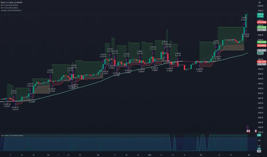
Pivot Percentile Trend - Strategy [presentTrading]
█ Introduction and How it is Different
The "Pivot Percentile Trend - Strategy" from PresentTrading represents a paradigm shift in technical trading strategies. What sets this strategy apart is its innovative use of pivot percentiles, a method that goes beyond traditional indicator-based analyses. Unlike standard strategies that might depend on single-dimensional signals, this approach takes a multi-layered view of market movements, blending percentile calculations with SuperTrend indicators for a more nuanced and dynamic market analysis.
This strategy stands out for its ability to process multiple data points across various timeframes and pivot lengths, thereby capturing a broader and more detailed picture of market trends. It's not just about following the price; it's about understanding its position in the context of recent historical highs and lows, offering a more profound insight into potential market movements.
BTC 6h L/S
Where traditional methods might react to market changes, the Pivot Percentile Trend strategy anticipates them, using a calculated approach to identify trend strengths and weaknesses. This foresight gives traders a significant advantage, allowing for more strategic decision-making and potentially increasing the chances of successful trades.
In essence, this strategy introduces a more comprehensive and proactive approach to trading, harnessing the power of advanced percentile calculations combined with the robustness of SuperTrend indicators. It's a strategy designed for traders who seek a deeper understanding of market dynamics and a more calculated approach to their trading decisions.
Local picture
█ Strategy, How It Works: Detailed Explanation
🔶 Percentile Calculations
- The strategy employs percentile calculations to assess the relative position of current market prices against historical data.
- For a set of lengths (e.g., `length * 1`, `length * 2`, up to `length * 7`), it calculates the 75th percentile for high values (`percentilesHigh`) and the 25th percentile for low values (`percentilesLow`).
- These percentiles provide a sense of where the current price stands compared to recent price ranges.
Length - 10
Length - 15
🔶 SuperTrend Indicator
- The SuperTrend indicator is a key component, providing trend direction signals.
- It uses the `currentTrendValue`, derived from the difference between bull and bear strengths calculated from the percentile data.
* used the Supertrend toolkit by @EliCobra
🔶 Trend Strength Counts
- The strategy calculates counts of bullish and bearish indicators based on comparisons between the current high and low against high and low percentiles.
- `countBull` and `countBear` track the number of times the current high is above the high percentiles and the current low is below the low percentiles, respectively.
- Weak bullish (`weakBullCount`) and bearish (`weakBearCount`) counts are also determined by how often the current lows and highs fall within the percentile range.
*The idea of this strength counts mainly comes from 'Trend Strength Over Time' @federalTacos5392b
🔶 Trend Value Calculation
- The `currentTrendValue` is a crucial metric, computed as `bullStrength - bearStrength`.
- It indicates the market's trend direction, where a positive value suggests a bullish trend and a negative value indicates a bearish trend.
🔶 Trade Entry and Exit Logic
- The entry points for trades are determined by the combination of the trend value and the direction indicated by the SuperTrend indicator.
- For a long entry (`shouldEnterLong`), the `currentTrendValue` must be positive and the SuperTrend indicator should show a downtrend.
- Conversely, for a short entry (`shouldEnterShort`), the `currentTrendValue` should be negative with the SuperTrend indicating an uptrend.
- The strategy closes positions when these conditions reverse.
█ Trade Direction
The strategy is versatile, allowing traders to choose their preferred trading direction: long, short, or both. This flexibility enables traders to tailor their strategies to their market outlook and risk appetite.
█ Default Settings and Customization
1. Trade Direction: Selectable as Long, Short, or Both, affecting the type of trades executed.
2. Indicator Source: Pivot Percentile Calculations, key for identifying market trends and reversals.
3. Lengths for Percentile Calculation: Various configurable lengths, influencing the scope of trend analysis.
4. SuperTrend Settings: ATR Length 20, Multiplier 18, affecting indicator sensitivity and trend detection.
5. Style Options: Custom colors for bullish (green) and bearish (red) trends, aiding visual interpretation.
6. Additional Settings: Includes contrarian signals and UI enhancements, offering strategic and visual flexibility.
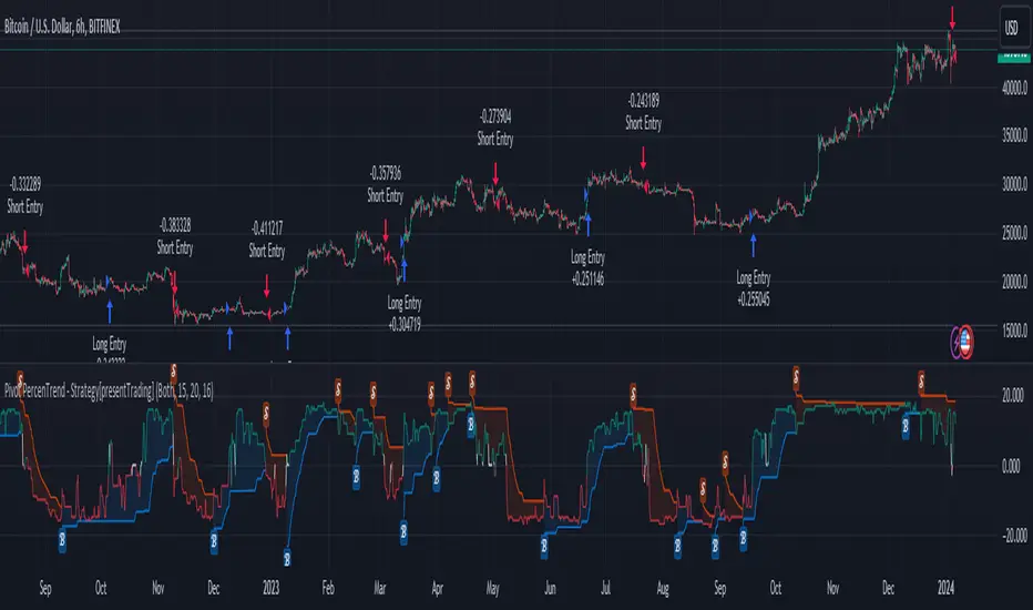
Session Breakout Scalper Trading BotHi Traders !
Introduction:
I have recently been exploring the world of automated algorithmic trading (as I prefer more objective trading strategies over subjective technical analysis (TA)) and would like to share one of my automation compatible (PineConnecter compatible) scripts “Session Breakout Scalper”.
The strategy is really simple and is based on time conditional breakouts although has more ”relatively” advanced optional features such as the regime indicators (Regime Filters) that attempt to filter out noise by adding more confluence states and the ATR multiple SL that takes into account volatility to mitigate the down side risk of the trade.
What is Algorthmic Trading:
Firstly what is algorithmic trading? Algorithmic trading also known as algo-trading, is a method of using computer programs (in this case pine script) to execute trades based on predetermined rules and instructions (this trading strategy). It's like having a robot trader who follows a strict set of commands to buy and sell assets automatically, without any human intervention.
Important Note:
For Algorithmic trading the strategy will require you having an essential TV subscription at the minimum (so that you can set alerts) plus a PineConnecter subscription (scroll down to the .”How does the strategy send signals” headings to read more)
The Strategy Explained:
Is the Time input true ? (this can be changed by toggling times under the “TRADE MEDIAN TIMES” group for user inputs).
Given the above is true the strategy waits x bars after the session and then calculates the highest high (HH) to lowest low (LL) range. For this box to form, the user defined amount of bars must print after the session. The box is symmetrical meaning the HH and LL are calculated over a lookback that is equal to the sum of user defined bars before and after the session (+ 1).
The Strategy then simultaneously defines the HH as the buy level (green line) and the LL as the sell level (red line). note the strategy will set stop orders at these levels respectively.
Enter a buy if price action crosses above the HH, and then cancel the sell order type (The opposite is true for a stop order).
If the momentum based regime filters are true the strategy will check for the regime / regimes to be true, if the regime if false the strategy will exit the current trade, as the regime filter has predicted a slowing / reversal of momentum.
The image below shows the strategy executing these trading rules ( Regime filters, "Trades on chart", "Signal & Label" and "Quantity" have been omitted. "Strategy label plots" has been switched to true)
Other Strategy Rules:
If a new session (time session which is user defined) is true (blue vertical line) and the strategy is currently still in a trade it will exit that trade immediately.
It is possible to also set a range of percentage gain per day that the strategy will try to acquire, if at any point the strategy’s profit is within the percentage range then the position / trade will be exited immediately (This can be changed in the “PERCENT DAY GAIN” group for user inputs)
Stops and Targets:
The strategy has either static (fixed) or variable SL options. TP however is only static. The “STRAT TP & TP” group of user inputs is responsible for the SL and TP values (quoted in pips). Note once the ATR stop is set to true the SL values in the above group no longer have any affect on the SL as expected.
What are the Regime Filters:
The Larry Williams Large Trade Index (LWLTI): The Larry Williams Large Trade Index (LWTI) is a momentum-based technical indicator developed by iconic trader Larry Williams. It identifies potential entries and exits for trades by gauging market sentiment, particularly the buying and selling pressure from large market players. Here's a breakdown of the LWTI:
LWLTI components and their interpretation:
Oscillator: It oscillates between 0 and 100, with 50 acting as the neutral line.
Sentiment Meter: Values above 75 suggest a bearish market dominated by large selling, while readings below 25 indicate a bullish market with strong buying from large players.
Trend Confirmation: Crossing above 75 during an uptrend and below 25 during a downtrend confirms the trend's continuation.
The Andean Oscillator (AO) : The Andean Oscillator is a trend and momentum based indicator designed to measure the degree of variations within individual uptrends and downtrends in the prices.
Regime Filter States:
In trading, a regime filter is a tool used to identify the current state or "regime" of the market.
These Regime filters are integrated within the trading strategy to attempt to lower risk (equity volatility and/or draw down). The regime filters have different states for each market order type (buy and sell). When the regime filters are set to true, if these regime states fail to be true the trade is exited immediately.
For Buy Trades:
LWLTI positive momentum state: Quotient of the lagged trailing difference and the ATR > 50
AO positive momentum state: Bull line > Bear line (signal line is omitted)
For Sell Trades:
LWLTI negative momentum stat: Quotient of the lagged trailing difference and the ATR < 50
AO negative momentum state: Bull line < Bear line (signal line is omitted)
How does the Strategy Send Signals:
The strategy triggers a TV alert (you will neet to set a alert first), TV then sends a HTTP request to the automation software (PineConnecter) which receives the request and then communicates to an MT4/5 EA to automate the trading strategy.
For the strategy to send signals you must have the following
At least a TV essential subscription
This Script added to your chart
A PineConnecter account, which is paid and not free. This will provide you with the expert advisor that executes trades based on these strategies signals.
For more detailed information on the automation process I would recommend you read the PineConnecter documentation and FAQ page.
Dashboard:
This Dashboard (top right by defualt) lists some simple trading statistics and also shows when a trade is live.
Important Notice:
- USE THIS STRATEGY AT YOUR OWN RISK AND ALWAYS DO YOUR OWN RESEARCH & MANUAL BACKTESTING !
- THE STRATEGY WILL NOT EXHIBIT THE BACKTEST PERFORMANCE SEEN BELOW IN ALL MARKETS !
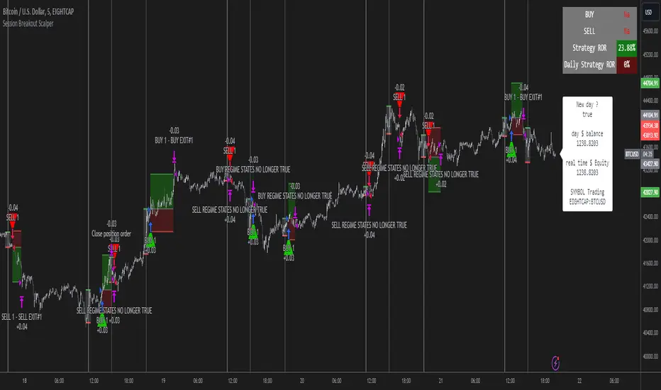
LuxAlgo - Backtester (PAC)The PAC Backtester is an innovative strategy script that allows users to create a wide variety of strategies derived from price action-related concepts for a data-driven approach to discretionary trading strategies.
Thanks to our 'Step' and 'Match' algorithm, users can create custom and complex strategy entries and exits from features such as market structure, order blocks, imbalances, as well as any external indicators, allowing users to create entries from a sequence of conditions and/or multiple matching conditions.
We included a complete alert system that will send a notification for each action taken by the strategy and we also allow users to set custom messages for each action taken by a strategy.
🔶 Features
🔹 Step & Match Algorithm
More complex entry rules can be created by using multiple conditions together, this is done thanks to the Step dropdown setting on the right of each condition.
The Step setting is directly related to the Step & Match algorithm and works in two ways:
When two or more conditions have the same step number, both conditions are evaluated. Used to test matching conditions.
When two or more conditions have different step numbers, each condition will be evaluated in order, testing for the first step and switching to the next step once the previous one is true. When the final step is true the strategy will open a market order. Used to create a sequence of conditions.
This operation is complementary, as you can create a sequence of conditions with one step consisting of two or more matching conditions as long as they have the same step number.
🔹 Fully Customizable Price Action Concepts As Entries
We allow the users to use market structures, order blocks, imbalances, and external sources together to set their custom entry and exit conditions.
Market structures are commonly used to determine trend direction by indicating when prices break prior swing points. Their occurrence can be used as entry conditions.
Order blocks highlight areas where institutional market participants open positions, one can use order blocks to determine confirmation entries or potential targets as we can expect there is a large amount of liquidity at these order blocks. Price entering, being within, or mitigating an order block can be used as an entry condition.
Market imbalances highlight areas where there is a disparity between supply and demand. Price entering, being within, or mitigating an imbalance can be used as an entry condition.
This system also allows the use of external sources to create entry and exit conditions, such as moving averages, bands, trailing stops...etc.
🔹 Complete Alert System
Users can get alerted for any action executed by a strategy, from opening positions to closing them.
The message field in the Alert Messages setting section allows for the strategy to send a custom alert message depending on the action taken by the strategy, if no messages are set the strategy will send default messages.
🔶 Usage
Users can create complete price action strategies from this script, let's see an example using the following entry conditions:
Long: Mitigated bearish order block occurring during the New York session after a mitigated bearish imbalance.
Short: Mitigated bullish order block occurring during the New York session after a mitigated bullish imbalance.
Take Profit: 2 points away from the entry price.
Stop Loss: 1 point away from the entry price.
We can also use features from Price Action Concepts™ to construct custom exit conditions, leading to the following strategy conditions:
Long: Bullish CHoCH and price mitigates bearish FVG.
Short: Bearish CHoCH and price mitigates bullish FVG.
Exit Long: Price mitigates bearish order block.
Exit Short: Price mitigates bullish order block.
Users can achieve a wide variety of results by using external indicators as an input source for entries and exits, combining the best from price action and technical indicators. We might for example be interested in exiting a position when the RSI oscillator is overbought or oversold.
🔶 Strategy Properties (Important)
This script backtest is done on daily EURGBP, using the following backtesting properties:
Balance (default): 10 000 (default base currency)
Order Size: 10% of the equity
Comission: 3.4 pips (average spread for EURGBP)
Slippage: 1 tick
Stop Loss: 0.01 points away from entry price
We use these properties to ensure a realistic preview of the backtesting system, do note that default properties can be different for various reasons described below:
Order Size: 1 contract by default, this is to allow the strategy to run properly on most instruments such as futures.
Comission: Comission can vary depending on the market and instrument, there is no default value that might return realistic results.
We strongly recommend all users to ensure they adjust the Properties within the script settings to be in line with their accounts & trading platforms of choice to ensure results from strategies built are realistic.
🔶 How to access
You can see the Author's Instructions below to learn how to get access.
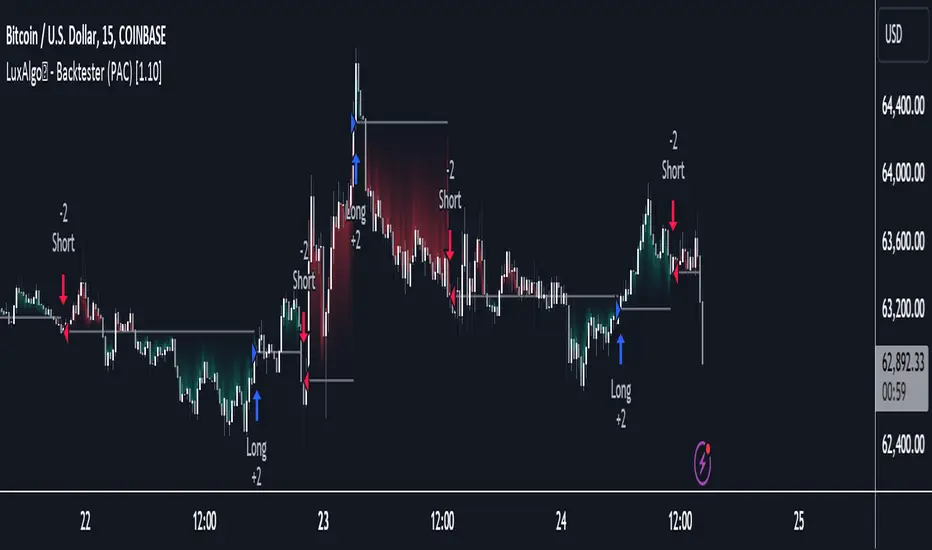
Long-Only Opening Range Breakout (ORB) with Pivot PointsIntraday Trading Strategy: Long-Only Opening Range Breakout (ORB) with Pivot Points
Background:
Opening Range Breakout (ORB) is a popular long-only trading strategy that capitalizes on the early morning volatility in financial markets. It's based on the idea that the initial price movements during the first few minutes or hours of the trading day can set the tone for the rest of the session. The strategy involves identifying a price range within which the asset trades during the opening period and then taking long positions when the price breaks out to the upside of this range.
Pivot Points are a widely used technical indicator in trading. They represent potential support and resistance levels based on the previous day's price action. Pivot points are calculated using the previous day's high, low, and close prices and can help traders identify key price levels for making trading decisions.
How to Use the Script:
Initialization: This script is written in Pine Script, a domain-specific language for trading strategies on the TradingView platform. To use this script, you need to have access to TradingView.
Apply the Script: You can do this by adding it to your favorites, then selecting the script in the indicators list under favorites or by searching for it by name under community scripts.
Customize Settings: The script allows you to customize various settings through the TradingView interface. These settings include:
Opening Session: You can set the time frame for the opening session.
Max Trades per Day: Specify the maximum number of long trades allowed per trading day.
Initial Stop Loss Type: Choose between using a percentage-based stop loss or the previous candles low for stop loss calculations.
Stop Loss Percentage: If you select the percentage-based stop loss, specify the percentage of the entry price for the stop loss.
Backtesting Start and End Time: Set the time frame for backtesting the strategy.
Strategy Signals:
The script will display pivot points in blue (R1, R2, R3, R4, R5) and half-pivot points in gray (R0.5, R1.5, R2.5, R3.5, R4.5) on your chart.
The green line represents the opening range.
The script generates long (buy) signals based on specific conditions:
---The open price is below the opening range high (h).
---The current high price is above the opening range high.
---Pivot point R1 is above the opening range high.
---It's a long-only strategy designed to capture upside breakouts.
---It also respects the maximum number of long trades per day.
The script manages long positions, calculates stop losses, and adjusts long positions according to the defined rules.
Trailing Stop Mechanism
The script incorporates a dynamic trailing stop mechanism designed to protect and maximize profits for long positions. Here's how it works:
1. Initialization:
The script allows you to choose between two types of initial stop loss:
---Percentage-based: This option sets the initial stop loss as a percentage of the entry price.
---Previous day's low: This option sets the initial stop loss at the previous day's low.
2. Setting the Initial Stop Loss (`sl_long0`):
The initial stop loss (`sl_long0`) is calculated based on the chosen method:
---If "Percentage" is selected, it calculates the stop loss as a percentage of the entry price.
---If "Previous Low" is selected, it sets the stop loss at the previous day's low.
3. Dynamic Trailing Stop (`trail_long`):
The script then monitors price movements and uses a dynamic trailing stop mechanism (`trail_long`) to adjust the stop loss level for long positions.
If the current high price rises above certain pivot point levels, the trailing stop is adjusted upwards to lock in profits.
The trailing stop levels are calculated based on pivot points (`r1`, `r2`, `r3`, etc.) and half-pivot points (`r0.5`, `r1.5`, `r2.5`, etc.).
The script checks if the high price surpasses these levels and, if so, updates the trailing stop accordingly.
This dynamic trailing stop allows traders to secure profits while giving the position room to potentially capture additional gains.
4. Final Stop Loss (`sl_long`):
The script calculates the final stop loss level (`sl_long`) based on the following logic:
---If no position is open (`pos == 0`), the stop loss is set to zero, indicating there is no active stop loss.
---If a position is open (`pos == 1`), the script calculates the maximum of the initial stop loss (`sl_long0`) and the dynamic trailing stop (`trail_long`).
---This ensures that the stop loss is always set to the more conservative of the two values to protect profits.
5. Plotting the Stop Loss:
The script plots the stop loss level on the chart using the `plot` function.
It will only display the stop loss level if there is an open position (`pos == 1`) and it's not a new trading day (`not newday`).
The stop loss level is shown in red on the chart.
By combining an initial stop loss with a dynamic trailing stop based on pivot points and half-pivot points, the script aims to provide a comprehensive risk management mechanism for long positions. This allows traders to lock in profits as the price moves in their favor while maintaining a safeguard against adverse price movements.
End of Day (EOD) Exit:
The script includes an "End of Day" (EOD) exit mechanism to automatically close any open positions at the end of the trading day. This feature is designed to manage and control positions when the trading day comes to a close. Here's how it works:
1. Initialization:
At the beginning of each trading day, the script identifies a new trading day using the `is_newbar('D')` condition.
When a new trading day begins, the `newday` variable becomes `true`, indicating the start of a new trading session.
2. Plotting the "End of Day" Signal:
The script includes a plot on the chart to visually represent the "End of Day" signal. This is done using the `plot` function.
The plot is labeled "DayEnd" and is displayed as a comment on the chart. It signifies the EOD point.
3. EOD Exit Condition:
When the script detects that a new trading day has started (`newday == true`), it triggers the EOD exit condition.
At this point, the script proceeds to close all open positions that may have been active during the trading day.
4. Closing Open Positions:
The `strategy.close_all` function is used to close all open positions when the EOD exit condition is met.
This function ensures that any remaining long positions are exited, regardless of their current profit or loss.
The function also includes an `alert_message`, which can be customized to send an alert or notification when positions are closed at EOD.
Purpose of EOD Exit
The "End of Day" exit mechanism serves several essential purposes in the trading strategy:
Risk Management: It helps manage risk by ensuring that positions are not left open overnight when markets can experience increased volatility.
Capital Preservation: Closing positions at EOD can help preserve trading capital by avoiding potential adverse overnight price movements.
Rule-Based Exit: The EOD exit is rule-based and automatic, ensuring that it is consistently applied without emotions or manual intervention.
Scalability: It allows the strategy to be applied to various markets and timeframes where EOD exits may be appropriate.
By incorporating an EOD exit mechanism, the script provides a comprehensive approach to managing positions, taking profits, and minimizing risk as each trading day concludes. This can be especially important in volatile markets like cryptocurrencies, where overnight price swings can be significant.
Backtesting: The script includes a backtesting feature that allows you to test the strategy's performance over historical data. Set the start and end times for backtesting to see how the long-only strategy would have performed in the past.
Trade Execution: If you choose to use this script for live trading, make sure you understand the risks involved. It's essential to set up proper risk management, including position sizing and stop loss orders.
Monitoring: Monitor the long-only strategy's performance over time and be prepared to make adjustments as market conditions change.
Disclaimer: Trading carries a risk of capital loss. This script is provided for educational purposes and as a starting point for your own long-only strategy development. Always do your own research and consider seeking advice from a qualified financial professional before making trading decisions.
